Activation Function for Hidden Layers in Neural Networks

In machine learning, a neural network consists of three layers: Input, Hidden and Output. Neurons in the hidden and output layers contain activation functions to ensure the model learns complex information from the data. The choice of these activation functions can dramatically change the results.

In our previous blog on activation functions, we learned about the definition, properties, and types of activation functions. In this blog, we will see the available options for hidden layer activation functions while designing neural network models.

Activation Function Choices for Hidden Layers

In a neural network, hidden layers are responsible for learning complex patterns present in the data. A network can have 0 or more hidden layers depending on how complex the dataset is. For example, in the case of image datasets, we need a significantly deeper network (including 10s of hidden layers to understand the complexities.

• A hidden layer takes input from the previous layer, which can be either a hidden or an input layer, and produces output for the next layer, which can be another hidden layer or an output layer.
• The first few layers of hidden layers, which are closer to the input layer, contain most of the learning from the overall learning through the entire dataset. The choice of a good activation function can dramatically influence this learning.

Usually, all hidden layers contain the same activation function, but there are provisions for defining it for every layer present as a hidden layer. For example, a neural network can have 10 hidden layers for which we need to define activation functions 10 times (or use the default activation function) for each layer.

We only use non-linear activation functions in hidden layers because of two significant advantages:

• Non-linearities help in extracting complex relationships present in data. A linear or no-activation function will act like a linear regression model.
• It allows us to stack multiple hidden layers to form the neural network architecture.

There are a lot of activation functions present in the literature, but here we will discuss some of the most frequently seen non-linear activation functions, and those are:

1. Sigmoid
2. Tanh
3. ReLU (Rectified Linear Unit)

Sigmoid Activation Function

Sigmoid is one of the first and most used activation functions used in hidden layers across multiple applications. In machine learning, we first encounter the Sigmoid function in Logistic Regression, where we try to classify samples into two categories using the logit function, which is nothing but a type of sigmoid function.

The mathematical formula for this activation function is:

sigmoid(X) = 1/(1 + exp(-x)), where x ∈ (-∞, + ∞).

This sigmoid function is monotonic (non-decreasing or non-increasing), and to calculate the range of this function, let's substitute the values of x as +∞ and -∞, then,

• sigmoid (+∞) = 1/(1 + exp(-∞)) = 1/(1 + 0) = 1, because exp = e ≈ 2.718.
• sigmoid (+∞) = 1/(1 + exp(+∞)) = 1/(1 + ∞) = 1/∞ = 0.

So, the output of the sigmoid activation function has a bounded range of (0, 1). Now, during the updation of parameters, optimizers try to find the derivative of the sigmoid function and the calculation for the same is given in the image below.

The plot for the gradient of the sigmoid function is shown in the image above. We can observe that the sigmoid gradient has significant values when x is between -3 to +3, and beyond that, it quickly decays to zero. Also, the gradient has only positive values, as the graph shows.

Let's try to implement this in Python.

from matplotlib import pyplot as plt
import numpy as np

## Function to calculate the sigmoid 
def sigmoid(x):
    sig = 1/(1+np.exp(-x))
    return sig

## Function to calculate the gradient of sigmoid based on calculation
def grad_sigmoid(x):
    sig = sigmoid(x) * (1 - sigmoid(x))
    return sig

x = [t for t in range(-10, 10)] ## Defining the input range to be [-10, 10]

y = [sigmoid(i) for i in x]
y_grad = [grad_sigmoid(i) for i in x]

plt.figure('Sigmoid Activation Function')
plt.plot(x, y, 'g', label='sigmoid')
plt.plot(x, y_grad, 'r', label='gradient')
plt.legend(loc='best')
plt.xlabel('X')
plt.show()

Don't worry, no one implements these things from scratch, and the support for these activation functions can be easily found in native libraries like tensorflow or keras. Let's see that example and compare the time taken by scratch implementation vs the Keras-implemented sigmoid function.

import tensorflow as tf
import time

x = [t for t in np.arange(-500.0, 500.0, 0.01)]

t1 = time.time()
out = tf.keras.activations.sigmoid(x)
total_time = (time.time() - t1)*1000
print("Total time taken by Keras implementation is ",total_time, " micro-seconds")

t1 = time.time()
out = [sigmoid(i) for i in x]
total_time = (time.time() - t1)*1000
print("Total time taken by scratch implementation is ",total_time, " micro-seconds")

## Total time taken by Keras implementation is 34.350 micro-seconds
## Total time taken by scratch implementation is 80.785 micro-seconds

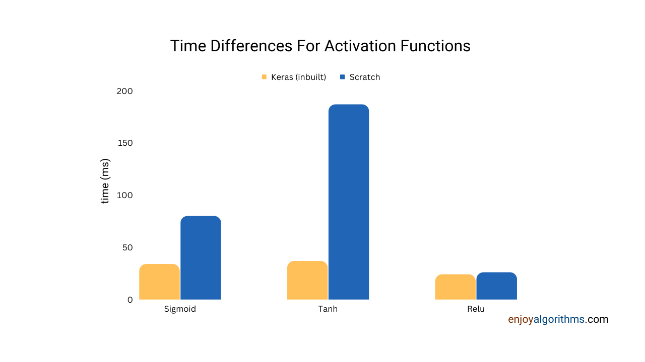
The time taken by the Keras implemented sigmoid function is way lesser than the scratch implementation. The reason is that frameworks use multiple optimization techniques to reduce the algorithm's time complexity for calculating the Sigmoid.

Key observations on Sigmoid

Advantages

1. The output of the Sigmoid lies in the range of (0, 1), making it a perfect candidate for separating classes or samples (either 0 or 1).
2. The gradient curve is smooth, which helps the model converge. 
3. Gradient calculation is very cheap and can be represented in terms of the original function.

Disadvantages

1. Gradient values quickly decay to zero, making the sigmoid activation function suffer from the Vanishing gradient problem. A vanishing gradient is a problem in neural networks where the updation of parameters stops affecting the cost function, and the model fails to learn.
2. The values of the Sigmoid are not zero-centred, and the values always remain positive. It makes training biased and unstable, requiring more epochs to train the model properly.
3. This activation function is computationally expansive because it involves the calculation of exponential.

Tips for using Sigmoid as an Activation Function in hidden layers

1. Input data should be normalized to [0, 1] for better performance.
2. We initialize the weight and bias values for the first time, and then optimization algorithms change these values based on the cost function values. Generally, this initialization is done randomly, but if our neural network architecture contains Sigmoid as an activation function, weight initialization should be done using Xavier Initialization, a.k.a Glorot Initialization. In this initialization schema, we initialize the bias values with zero and weight values as:

initializer = tf.keras.initializers.GlorotNormal()
layer = tf.keras.layers.Dense(3, kernel_initializer=initializer)

For more details, please see these references:

1. https://keras.io/api/layers/initializers/
2. https://paperswithcode.com/method/xavier-initialization

Tanh Activation Function (Hyperbolic Tangent)

ML researchers wanted to solve the unstable training issue present in the Sigmoid. They designed another activation function similar to the Sigmoid but having zero-centeredness, which became more popular.

The mathematical formula for this activation function is:

tanh(x) = (exp(x) - exp(-x))/(exp(x) + exp(-x)), where x ∈ (-∞, + ∞).

Tanh is also a monotonic activation function defined for all the real numbers. Let's see the range of this function by substituting the values of x as -∞ and +∞.

tanh(-∞) = (exp(-∞) - exp(∞))/(exp(-∞) + exp(∞)), as exp(-∞) ≈ 0, and 2∞ ≈ ∞
         = (exp(-2∞) - 1)/(exp(-2∞) + 1) = (0-1)/(0+1) = -1

tanh(∞) = (exp(∞) - exp(-∞))/(exp(∞) + exp(-∞)), as exp(-∞) ≈ 0, and 2∞ ≈ ∞
         = (1-exp(2∞))/(1+exp(-2∞)) = (1-0)/(1+0) = 1

So, the tanh activation function range is (-1, 1) and zero-centred. If we observe, tanh is nothing but 2sigmoid (2x) — 1. So, it contains all the properties of the Sigmoid function but with an improved thing of zero-centeredness. Now, for any activation function, its gradient plays an essential role in the updation of parameters, so let's see the curve for that.

The graph shows that tanh is crossing the origin, and the gradient curve is smoother. Let's implement it using Python.

from matplotlib import pyplot as plt
import numpy as np

## Function to calculate the tanh 
def tanh(x):
    tan = (np.exp(x) - np.exp(-x))/(np.exp(x) + np.exp(-x))
    return tan

## Function to calculate the gradient
def tanh_grad(x):
    return (1 - tanh(x)**2)

x = [float(t) for t in range(-10, 10)]

y = [tanh(i) for i in x]
y_grad = [tanh_grad(i) for i in x]

plt.figure('Sigmoid Activation Function')

plt.plot(x, y, 'g', label='tanh')
plt.plot(x, y_grad, 'r', label='gradient')
plt.legend(loc='best')
plt.xlabel('X')

plt.show()

Tanh activation function support can be easily found in frameworks and libraries used to build neural networks. For example, in Keras:

## out = tf.keras.activations.tanh(x)

## To calculate the time difference between scratch implementation, we can follow the same method

import tensorflow as tf
import time

x = [t for t in np.arange(-500.0, 500.0, 0.01)]

t1 = time.time()
out = tf.keras.activations.tanh(x)
total_time = (time.time() - t1)*1000
print("Total time taken by Keras implementation is ",total_time, " micro-seconds")

t1 = time.time()
out = [tanh(i) for i in x]
total_time = (time.time() - t1)*1000
print("Total time taken by scratch implementation is ",total_time, " micro-seconds")

## Total time taken by Keras implementation is 37.160 micro-seconds
## Total time taken by scratch implementation is 187.885 micro-seconds

Note: Please observe the difference in time required to calculate the same tanh function from scratch versus the Keras implementation.

Key observations on Tanh

Advantages

1. The gradient curve is smoother, which helps the model converge.
2. Zero-centeredness increases the stability while training models.
3. The bounded nature of tanh in the range of (-1, 1) makes it a perfect candidate for segregating the samples even further in case of classification problems.
4. Gradient calculation is more straightforward as it can be directly represented in terms of the original function.

Disadvantages

1. The gradient function quickly decays to zero, as we saw in the Sigmoid. This raises the problem of vanishing gradient, and the model sometimes fails to learn.
2. The tanh function involves the calculation of the exponential function, which is computationally complex.

Tips for using Tanh as an Activation Function in hidden layers

1. Input data should be normalized to [-1, 1] before feeding to the neural network.
2. Similar to Sigmoid, weight initialization should be done using Xavier Initialization.

ReLU (Rectified Linear Unit) Activation Function

ReLU activation function has become the new common and most popular function in the neural network and deep learning architecture. Most famous libraries or frameworks have started using it as a default activation function for hidden layers. The reason for all this charm is that it is computationally very cheap, which makes it 6 to 7 times faster in terms of model convergence compared to the sigmoid and tanh activation functions.

The mathematical formula for the ReLU activation function is:

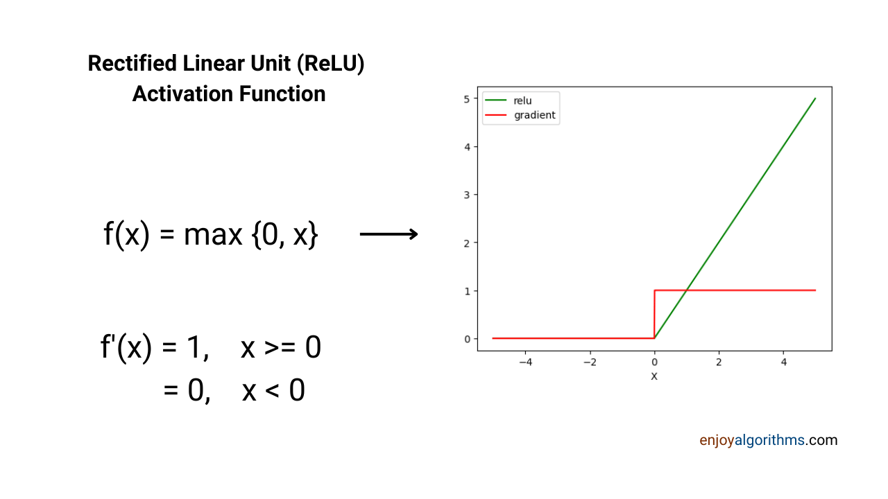
relu(x) = max{0, x}, where x ∈ (-∞, + ∞).

We can find that the range of this activation function would be [0, ∞). It was first discovered in 1975, but ML researchers started using it very late in 2010. This late adaptation is due to the rigid assumption to follow the differentiability. Let's discuss this in detail by looking at this function's curve and its derivative.

If we are familiar with the differentiability theory, we might have got that ReLU is not differentiable at x = 0. But differentiability is one of the fundamental properties for an activation function to hold. Then how does Relu become such a famous and valuable activation function if it is not differentiable?

The assumption of strict differentiability became a hurdle and the reason for the late adaption of Relu in Machine Learning. Yes, ReLU is not differentiable at x = 0, but in practice (or while coding), we can define the derivative of ReLU when x is 0. It will solve the issue of non-differentiability at one point. Let's see it through Python code.

from matplotlib import pyplot as plt
import numpy as np

def relu(x):
    return max(0, x)

def grad_relu(x):
    if x > 0:
        return 1
    else:
        return 0

x = [t for t in np.arange(-5.0, 5.0, 0.01)]
y = [relu(i) for i in x]
y_grad = [grad_relu(i) for i in x]

plt.plot(x, y, 'g', label='relu')
plt.plot(x, y_grad, 'r', label='gradient')
plt.legend(loc='best')
plt.xlabel('X')

plt.show()

Now, let's compare the time Keras implemented and the scratch-implemented ReLU.

x = [t for t in np.arange(-500.0, 500.0, 0.01)]
t1 = time.time()
out = tf.keras.activations.relu(x)
total_time = (time.time() - t1)*1000
print("Total time taken by Keras implementation is ",total_time, " micro-seconds")

t1 = time.time()
y = [relu(i) for i in x]
total_time = (time.time() - t1)*1000
print("Total time taken by scratch implementation is ",total_time, " micro-seconds")

## Total time taken by Keras implementation is 24.56 micro-seconds
## Total time taken by scratch implementation is 26.314 micro-seconds

Please observe one key point here, the time difference between the scratch-implemented and keras-implemented is not too huge, as we saw in the case of the sigmoid and tanh activation functions. This simplicity and extremely cheap computational requirement is the main reason for the popularity of ReLU. Researchers based on several experiments observed that using ReLU makes the model converge 6x to 7x times faster when compared to tanh or Sigmoid.

Key observations from the relu activation function

Advantages

1. It is computationally very cheap because of its linear nature.
2. The range of the ReLU function is [0, ∞), which means it is unbounded with a constant gradient of 1. So, if we have used ReLU as an activation function in our neural network, it can never face the vanishing gradient problem.

Disadvantages

1. It is not zero-centred, making training slightly unstable and requiring more iterations to train on for better performance.
2. It completely removes the negative values from the calculation making those neurons inactive. Suppose a case where the weight multiplication and bias addition will always output a negative value irrespective of the input values. Here, the entire network architecture will fall into a dead state, known as dead relu.
3. ReLU is unbounded, which helps solve the vanishing gradient problem, but it becomes prone to exploding gradient issues if weight or bias values have a higher magnitude.

Many more activation functions are present today that have improved and solved the problems of native relu, but we will discuss them in a separate blog.

Tips for using ReLU as an Activation Function in hidden layers

1. The input data should be normalized in the range of [0,1] to make sure that even if weight and bias values have greater magnitude, the multiplication will give a chance to avoid exploding gradient. 
2. The weight initialization should be done using the He uniform initializer, also known as the Kaiming initializer. Here, Biases are initialized with a zero and weight with Gaussian distributed random samples having a standard deviation of 2/nl, n represents the number of connections present in the layer l. Please see the image to observe the difference between He and Xavier's initialized weights in the case of the ReLU activation function.

initializer = tf.keras.initializers.HeUniform()
layer = tf.keras.layers.Dense(3, kernel_initializer=initializer)

Time Comparison for Sigmoid Tanh and Relu

The plot below shows the difference in the time required to calculate the different activation functions for the same input. It indicates that the ReLU requires significantly less time compared to others.

When to choose which activation function in the hidden layer?

Based on the above discussion, we learned that every activation function has certain advantages and disadvantages, which depend on our requirements. If we observe the timeline of these activation functions considered as the default activation function, it will tell us a lot about their age of popularity.

For example, Sigmoid was the default activation function for designing perceptrons until the 1990s. After the 1990s, till 2010, tanh was the default activation function, and after 2010, relu became the default one. 

Recent popular networks like Convolution Neural Networks and multi-layer perceptrons used for building trending machine learning applications use ReLU as their activation function. At the same time, recurrent networks like LSTM, GRU, or RNN, popularly used in time-series applications or forecasting techniques, use Sigmoid and Tanh activation functions.

If choosing these activation functions does not provide us with better results, we are still trying to decide which activation will best suit our neural network. The golden rule would be to apply different activation functions directly and observe the results to choose the best. As a summary:

1. Convolution Neural Networks: Use the ReLU activation function.
2. Multi-layer perceptrons or General ANN: Use the ReLU activation function.
3. Recurrent Neural Networks: Sigmoid or Tanh activation functions.

That's it for this blog. In the next blog, we will discuss the possible options of activation functions for the output layer and learn how to choose the best activation function.

Possible Interview Questions on the activation functions for hidden layers

These are some of the most asked interview questions on this topic:

1. Why did you choose Relu (or Sigmoid or tanh) activation function for your model?
2. What are Xavier and He initialization, and when to choose which initialization technique?
3. Why is ReLU faster than other activation functions?
4. What are the disadvantages of the ReLU activation function?
5. Where do we use the Sigmoid and Tanh activation functions?
6. Why is it preferred to use Keras' inbuilt activation functions instead of writing from scratch?

Conclusion

In this article, we discussed the important activation functions used in the hidden layer of neural networks. We learnt their scratch implementation and observed their time difference with the Keras implemented functions. Finally, we discussed how we could decide which activation would be the best to pick based on our network type. Our next blog will discuss options for activation functions for the Output layer. We hope you find the article enjoyable.