Data Pre-processing of Structured Data in Machine Learning

Introduction

Nowadays, data collection is one of the most common trends among organizations. Every company collects data for a variety of uses.

• Facebook collects data about our likings and dislikings.
• Amazon collects our data about our shopping patterns.
• Myntra collects our data about what we love to wear and many more.

Similarly, every firm is collecting data in some form. But interestingly, most of these firms are piling up millions of gigabytes of data without adequately utilizing it. The reason is there is a FOMO (Fear of Missing Out). What if they did not collect some data and later learned that it was necessary. So they record all potential properties with the belief that they will use them in the future. When they record any form of data, it comes with various impurities. These impurities need to be removed from our dataset to make them useful for machine learning or deep learning tasks. In this article, we will discuss steps used for the same.

Key takeaways from this blog

• What is the meaning of data?
• What are attributes?
• What are categorical and numerical features?
•  What is the need for data pre-processing techniques?
• What are the data pre-processing steps for structured data?
• Why do we need to scale the attributes?
• Splitting of data in three sets of train/validation/test.
• Some popular interview questions on this topic.

What are Data and Attributes?

Meaning of data

If we define the term “data” properly: Data is raw qualitative or quantitative information stored in numerical, textual, audible, or visual form. Based on this definition, we can have four different data formats:

• Numerical: Data present in the numerical format. E.g., Recording day-wise temperatures of our city (like 24°C, 24.7 °C), speed of the car (80 kmph, 92.5 kmph), etc.
• Textual: Data stored in the text format. E.g., Our emails, social media posts, movie reviews, etc.
• Visual: Data stored in the image or video format. E.g., Our profile photos, photos present on the social media post, etc.
• Audio: Data stored in the audio format. E.g., Our call records, our voice mails, etc.

The types of data

All the formats mentioned above can be categorized into two types:

• Structured Data: Data that contains a well-defined structure in it. This type of data is generally stored in the database or tabular form, e.g., numerical data recorded in excel sheets or CSV files. 
• Unstructured Data: Data that does not have any predefined form. E.g., Audio signals do not come with predefined properties. Similarly, email images are also considered unstructured data.

In this article, we will keep our discussion limited to structured datasets.

What are attributes?

While performing the data collection process for structured data, we usually observe and record the values of many individual properties for any phenomenon in a database. This unique, measurable property is termed an attribute in machine learning. For example, we want to build a machine learning model to sense whether there will be rain today. For that, we started recording the properties like atmospheric pressure, temperature, humidity, etc. Suppose we recorded this data in the tabular format shown in the image below.

Every individual property is recorded in each column, known as an attribute. And every row corresponds to one sample of data that records the values of different attributes for a particular instance.

Types of Attributes

Categorical or Qualitative Attributes

In this category, attributes can take values from a fixed, defined set of values. For example, weekday can take values from the set of {Monday, Tuesday, Wednesday, Thursday, Friday, Saturday, Sunday} and hence we can say that weekday is a categorical attribute. Similarly, if any attribute can take only a boolean value, i.e., from the set {True, False} or {0, 1}, then that attribute can be considered as a categorical attribute.

This set is further categorized as:

• Nominal: If we can apply a tag to the data, or simply say if we can brand it. Color can be tagged as red, white, black, etc.
• Ordinal: If we can order the categories, like hot hotter, and hottest can be put in the desired order.

As we saw in the weekday example above, the defined set of categorical variables can contain non-numeric values. But, we know that our machines can not understand these values (text like weekdays), so we need to transform these attributes into a machine-readable format. One of such methods is one-hot encoding, using which seven days can be converted as seven attributes, like Monday = (1, 0, 0, 0, 0, 0, 0); Tuesday = (0, 1, 0, 0, 0, 0, 0) and so on.

Numerical or Quantitative Attributes

In this category, values of the recorded phenomena are either discrete or continuous but real-valued. For example, the Vehicle’s Speed, Battery’s Current are numerical attributes.

This category is further categorized as:

• Discrete: Attributes in the countable format, for example, 1,2,3,4, etc.
• Continuous: Attributes that we record using measurement techniques like Vehicle speed, weather temperature, etc.

What is the need for data pre-processing?

One important word that we missed in the definition of data is “raw”. The data we record comes to us in the raw form of data. We know that the petrol we use to run our vehicles comes from the raw form of petroleum oil. We process that raw form, remove impurities, and extract valuable things from it. Because of these impurities, we can not use them directly to run the vehicle.

In the same fashion, data is the new oil in the IT industry. The data we receive from the natural data-collection process contains various impurities. Hence, it can not be directly used to build or train machine learning models. Raw data may have outliers, unwanted attributes, missing values, and many other complex challenges. Hence we need to refine this into some meaningful form. The process of this transformation can be termed data-preprocessing. If we properly define the data pre-processing term,

“Data pre-processing techniques generally refer to the addition, deletion, or transformation of data.”

Now that we know what data preprocessing is and the primary reason to use data preprocessing, let's quickly move ahead and look at some standard methods included in this process.

Data pre-processing steps for structured data

We collected different attributes, but using all of them can be too much for the model-building process. We need to leave out some attributes based on our problem domain understanding. Suppose theory says the temperature is not so important to decide whether there will be rain today. So, we will drop the temperature from our final set of attributes. 

We can not use every attribute we recorded to build our model. But we record as many attributes as we can. Can you guess why?

The combination of attributes is decided as per the project’s need. It may be possible that one attribute does not make any sense for one project, but for another, it becomes essential. So intuitively, our first step should be selecting the required attributes from the bulk of available attributes to solve the given problem. Once selected, these attributes are known as Features. In this article, we will learn five crucial pre-processing steps shown in the image below.

Step 1: Feature Selection

This step requires a small amount of domain knowledge of the problem statement. For example, suppose we train a machine learning model to predict the battery’s remaining life (For how many cycles we can recharge the battery). In that case, from the electrical domain knowledge, we can say that the features like Current (I), Voltage (V), and Temperature(T) patterns while charging and discharging the batteries will be helpful because these features derive the factor of aging of the battery.

But one central question we might be thinking, how did we know that these features will contribute to the battery’s aging? This intuition came from domain knowledge or research in that field. Another example could be that if the problem is related to estimating the energy produced by wind turbines, we should know critical factors that control wind energy production.

Generally, firms try to collect as many attributes as possible because having extra things does not hurt, but missing essential features can force reiterating the entire data collection process.

Several statistical methods or algorithms can help us find which attributes contribute the most and select those attributes as the set of features.

• Wrapper methods: For a given Machine Learning model, try out several combinations of attributes to check which combination is producing the best results (better accuracy or lesser error).
• Filter Methods: Statistical methods to check which attributes can affect the model the most and select the combination of those attributes.
• Embedded Methods: It is similar to wrapping methods, but this is more related to model building and internally checking the accuracy. Differences will be clear from the image below.

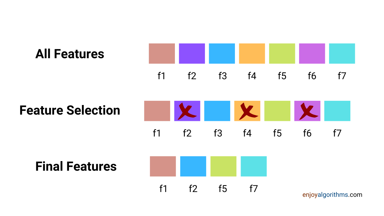
If we consider data in the form of rows and columns, then Columns represent the features (or attributes), and rows represent the values of those features. Feature selection is performed on the columns, not on rows.

Step 2: Feature Value Quality Assessment

In this step, we evaluate the quality of the data features. During the data collection process, it may be possible that some sensors stop working or get affected by noises, or in the case of human intervention, there can be some inconsistency related to the scale or measurement units. There is one famous line that says: It is simply unrealistic to expect that the data will be perfect.

Some famous impurities (aka anomalies) present in the data

Missing Values

Some rows may contain either no values or NaN (Not a Number) values. A similar thing can be observed in the image above. To tackle this problem, there are two solutions:

1. Eliminate Rows: We can simply delete the rows having missing or NaN values. But suppose the first column is the time feature, which shows that data was collected at that particular time. If we need data at a fixed sampling rate (the time difference between two consecutive samples to be consistent), this method will create problems. Right?

2. Estimate Rows: We can estimate the missing values in the rows using various techniques like:

• Linear interpolation: Fit a linear curve on the feature and estimate the missing values by the values on that line.

• Forecast modeling: Make a machine learning model that predicts the missing value based on the available values.
• Forward filling: Fill in the exact value of previously recorded data.
• Backward filling: If we know the last rows, fill the gaps with later values.
• Average filling: Fill the average value in place of NaN or missing values.

Wrong/ Inconsistent Values

These inconsistencies are better resolved with the help of human cross-checking. We can use some programming techniques to cross-check whether the data is consistent, but this is infeasible because of the 100s and 1000s of corner cases that can be present. Suppose the speed range for a motorbike can be in the range of 0 to 300 Km/h. But what if it is giving values in the range of 1000–5000 Km/h. We usually represent features graphically and manually resolve such errors.

Duplicate Values

Because of various factors, it may be possible to have duplicate values present in the data. It can make our model biased towards this duplicity as the model will see these repeated samples repeatedly. These anomalies can be removed with the help of graphical or statistical observations.

Presence of Noise

Sensors collecting data can have multiple forms of disturbances or noises. These noises are random and hence bring inconsistency in the data. Several filtering techniques can be used to denoise the signals, like Savitzky–Golay filter shown in the GIF below. These filters remove the jitter and smooth out the observations. Suppose the blue line is our data which has inconsistent spikes. We applied a filter that removed the spikes and transformed our data into dotted plots shown in the image.

Presence of Outliers

Outliers are the observations that lie at an abnormal distance from other values present in the random sample of the dataset. The decision of “what is abnormal” depends upon the data scientists working on that data. Several techniques are used to remove outliers from the dataset, like replacing outliers from the mean of data.

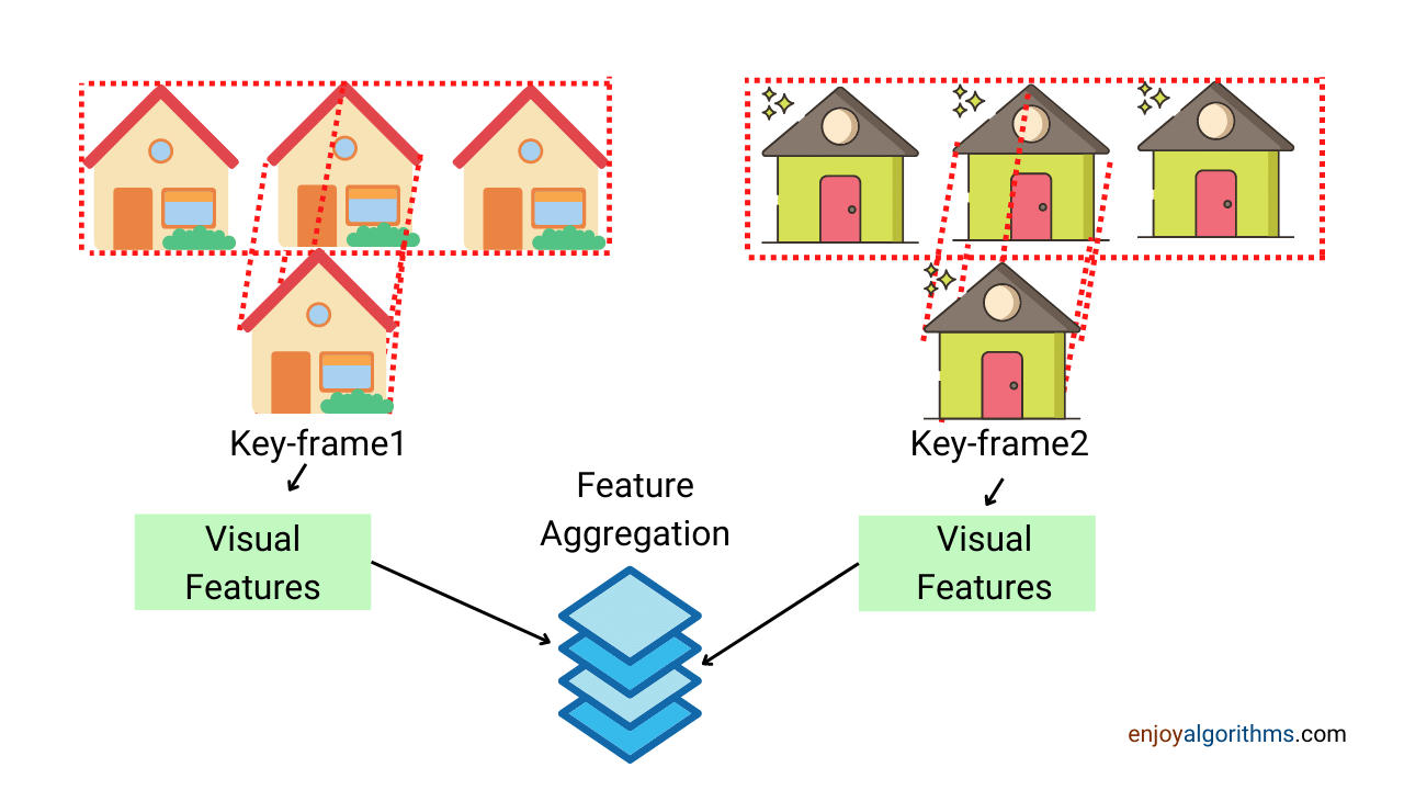
Step 3: Feature Aggregation

At the start of this blog, we discussed that data collection is a common trend nowadays. Following this trend, people have started collecting every minute of data. But suppose if some attribute is not required with that higher frequency, but still, we are collecting it. Storing and using all this data is computationally very expansive. That’s where we need aggregation.

For example, suppose one company collects the precipitation of waste materials from a water source every hour and collects it for years. Instead of every hour, we could have used monthly or daily precipitation data for a more straightforward visualization. This process is known as the aggregation of features. In a one-liner, we can say: Applying an aggregation function on raw data is feature aggregation. We extract desired rows here and then stack them to make the final data.

Step 4: Feature Sampling

Sampling is one of the crucial concepts in the data processing technique, which means creating subsets of data to perform specific actions on them or visualize them better. It means breaking big data into smaller chunks so that analysis becomes easy.

In real-life scenarios, because of sensor failure or human mistakes, it may be possible that different features have different sampling rates. Also, if we consider using all the data samples present in the raw data, it may be too expansive computationally.

Let’s consider one scenario where there are two machine learning models:

1. A light model that gives the predictions very fast. But it requires a considerable amount of data to achieve higher accuracy.
2. A complex model that takes slightly higher time than the light model. It can not be fed with massive data because of the limitation of computational power. Still, if less but meaningful information is given to this model, it can quickly achieve the accuracy of the first model.

Which model would you prefer?

The second one, right? So sampling of features gives us the ability to select the second model. We break data into meaningful samples and then use the samples having better meaning.

But the major challenge in the feature sampling step is that we must not lose valuable information. The varying sampling rates (In the classification problem of detecting cats and dogs in images, out of 100 image data, 90 images contain cats.) cause an imbalance among features, which means one feature has more samples than others. This imbalance can cause bias in the training data.

Sampling techniques help in reducing this imbalance present in the data.

Some famous sampling techniques

• Upsampling/Downsampling
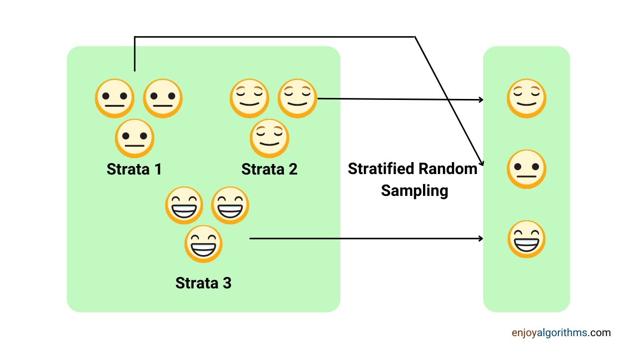
• Stratified Sampling
• Simple Random sampling
• Gaussian sampling

Feature sampling is also performed on the rows, but it is different from aggregation techniques. In the sampling step, we decide to increase or decrease the number of rows. But in aggregation, we always reduce the number of rows.

Let’s take one example to understand it clearly. Suppose we have 100 image data containing three objects: 1. Cat (50 images) 2. Dog (40 images) and 3. Apple (10 images). All three classes are not present in equal proportion, making our model biased towards Cat and Dog, and even apple will get classified as either Cat or Dog.

• Suppose we want to remove the apple class. Here we will perform the feature aggregation step, where we will extract rows corresponding to cats and dogs and then stack them to form the final data.
• Suppose we can not remove the apple class, and we want our model to predict all three categories. But we have imbalanced data. Hence we will perform the feature sampling step here. Upsampling the Apple class images and matching the quantity in which Cat and Dog class images were present will help.

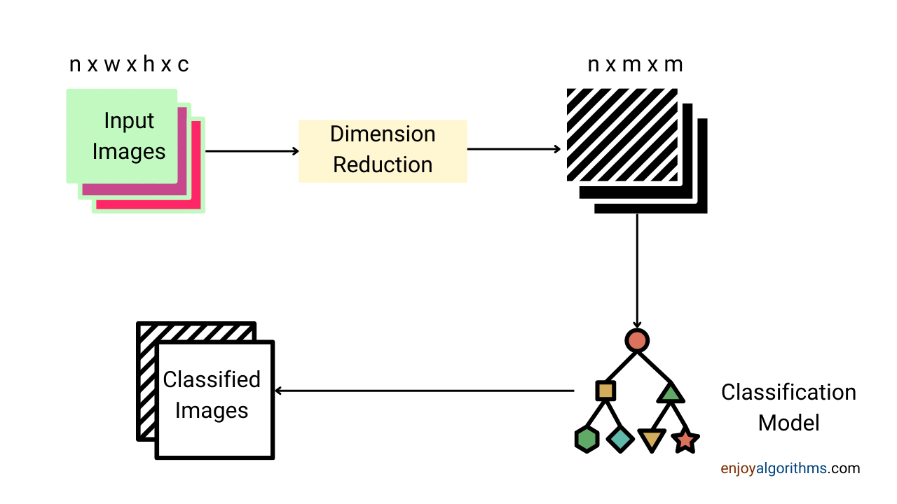
Step 5: Dimensionality Reduction

After gaining experience or getting advice from a domain expert, we can extract useful features from the sea of available features. But, as we mentioned, firms try to capture as many possible attributes; hence, there are too many features in the real-world dataset, and using all of them is infeasible. Let’s take an example to understand it better. Companies collect data for the vehicle’s speed and acceleration. From the domain knowledge, we know that both features are essential, but the question is: Do we really need speed and acceleration to be present in the final set?

Increasing the number of features brings the complexity factor with it. Every feature can be considered a separate dimension, and visualization (plotting features with respect to each other) will become more complex. Suppose we observe that “speed” and “acceleration” are highly dependent or correlated. In that case, we can choose just one and drop the other from the final set of attributes because we are not getting much extra information by keeping both of them. But what if we don’t have much information on which one to select and which one to discard?

In such scenarios, we take the help of dimensionality reduction techniques which aim to transform our features into a lesser number of features by maintaining as much information as possible. Some famous techniques for that are:

• PCA (Principal Component Analysis)
• High Cross-correlation
• t-SNE 

Reducing dimensionality helps in:

• Explainability in machine learning models
• Easiness for data pre-processing algorithms
• Better visualization

How is dimensionality reduction different from feature selection?

Removing features from the whole set of attributes is also a dimensionality reduction. But this process has certain limitations. It can be possible that we may not remove some features altogether. Here, the solution becomes challenging. We can not even keep them and can not even remove them. Then we need to make new attributes that contain maximum information from the original attributes.

We have done hands-on for all the steps mentioned above in this blog. Please have a look for a better understanding.

Why do we need to scale attributes?

These attributes are advised to scale before feeding to the machine learning model. But what do we mean by scale? Suppose we measure individual attributes of the same phenomena, which is driving the vehicle. One attribute is speed, which varies between 30 KMPH to 90 KMPH (max value is 90 and min value is 30), and another attribute is the distance varying from 5000 KM to 10000 KM (max value is 10000 and min value is 5000). If we want to observe the actual effect of these attributes on our machine learning model, we need to bring both these attributes in the same range variations ( for example, max value 1 and min value 0).

There are several methods available for this,

• Min-max normalization
• Z-mean normalization
• Exponential normalization, etc.

These are widely used scaling techniques for scaling the features. Detailed methods and the need for scaling are discussed in this blog.

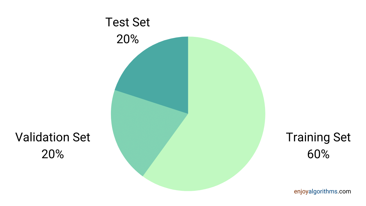
Splitting the dataset

After the steps mentioned above are done, we can say that we can use it directly for the machine learning model. But it is advised to split the data into three sets before feeding it to the model,

1. Training Set
2. Validation Set
3. Testing Set

Training Set: This set of data is used to train the model. The model learns the relationship between the input and output data or even among the input features present in the training dataset.

Validation Set: This set is used to validate model learning from the training dataset and tune the hyperparameters involved in the learning.

Test Set: This set is used to evaluate the model performance when used in real-world data. This set is entirely unseen to the model before actually being tested.

After knowing these three sets, one question should come to our mind: What is the ratio of the split in which we should divide the whole dataset into train/validate/test sets? The answer to this question is not fixed. One can choose the ratio as per the need. But, it is always advisable to use more training data so that our machine learning model will get exposure to all the corner cases. Based on different famous courses on Machine learning and Deep Learning, it is proposed that the optimal split ratio can be 3:1:1, I.e., 60% of the total dataset can be used in the training set, 20% as the validation set, and the rest 20% as test data. This is not hard and fast and can vary as per the need.

Let’s think over an open-ended question, and please send your thoughts in the comment /mail section: If everyone is collecting this gigantic amount of data, will it be considered Digital Junk in the near future?

Possible Interview Questions

• What is data preprocessing, and why do we need it?
• How do we check the quality of the data?
• How does feature sampling help?
• Is it necessary to remove outliers?
• Suppose you don't have the domain knowledge. How will you approach the feature selection step?
• Does dimensionality reduction help data visualization, or does it also transform the data?

Conclusion

This article has studied the fundamental data pre-processing techniques frequently used in Machine Learning and Data Science fields. Concepts like feature types, selection, quality assessment, aggregation, and dimensionality reduction are discussed in this blog. We hope you enjoyed these fundamentals.

Enjoy Learning, Enjoy Algorithms!