Time Series Forecasting: Statistical Model to Predict Future Values

Time Series is a set of observations taken at a specific periodic time. Time Series Forecasting refers to the use of statistical models to predict future values using the previously recorded observations. It is broadly classified into two parts:

• Univariate Time Series Forecasting: Involves a single variable
• Multivariate Time Series Forecasting: Involves multiple variables

Building a Statistical Forecasting model often involves a standard procedure. The image below depicts the steps to be carried out to build a forecasting model. We will use the ARIMA algorithm for this tutorial, which is extensively used in short-run forecasts.

Let’s dive into data analysis:

Data Analysis

For this tutorial, we will be using the Air Passenger Dataset available on Kaggle. It is a reasonably simple time-series data with “Timestamp” and “Number of passengers” as features. It contains approximately 144 rows and covers 11 years of passenger count.

Let’s take a look at the trend.

import pandas as pd
import plotly.express as px

air_passengers = pd.read_csv('AirPassengers.csv')

fig = px.line(air_passengers, x='Month', y="Passengers")
fig.show()

Time Series Decomposition

Understanding a whole time series could be a challenging task. Fortunately, the time series can be decomposed into a combination of trend, seasonality, and noise components. These components provide a valuable conceptual model for thinking about a time series prediction.

• Additive Decomposition: Assumes that the time series is a linear combination of Trend, Seasonality, and Residual.

• Multiplicative Decomposition: Assumes that the time series is a product of Trend, Seasonality, and Residual component.

The additive decomposition model is preferred when the seasonal variation is somewhat constant over time, while the multiplicative model is useful when the seasonal variation increases over time. For a concrete understanding, visit this blog. A multiplicative time series can be converted into an additive series using a log transformation. 

Yt = Tt x St x Rt
log(Yt) = log(Tt) + log(St) + log(Rt)

In our case, the seasonality increases over time, so we have to use a multiplicative time series decomposition. Let’s decompose our time series!

from statsmodels.tsa.seasonal import seasonal_decompose

decomposed = seasonal_decompose(series, model='multiplicative')

decomposed.plot()

From the above time series decomposition, we can infer that the time series has a seasonality period of 1 year, and the trend is strictly increasing. We also have some residuals or noise in the data, which we will attempt to resolve later.

Stationary Test

Before applying any forecasting models to a time series dataset, the time series needs to be stationary. A time series is said to be stationary if its statistical properties (mean, variance, & autocorrelation) do not change over time by a far value. It is clear from the above time series plot that the mean of our time series is increasing over time. We know it is not stationary but let’s just confirm it.

Several methods are available for testing the stationary nature of a time series. One such method is Dickey-Fuller Test.

Note: If the time series is not stationary, we can prove that the standard assumptions for forecasting analysis will not be held valid.

Dickey-Fuller Test:

The Dickey-Fuller test is a statistical significance test, which will give results in hypothesis tests. The hypothesis test considers a Null and an Alternative hypothesis. The hypothesis made for the Dickey-Fuller Test is as follows:

Null Hypothesis (H0): The time series is not stationary.

Alternate Hypothesis (Ha): The time series is stationary.

In the null hypothesis, we first consider that time-series data is non-stationary and then calculate the Dickey-Fuller Test (ADF) value. If the test statistics of the Dickey-Fuller Test (ADF) is less than the critical value(s), then reject the null hypothesis of non-stationary (Series is stationary). On the contrary, if the ADF is greater than the critical value(s), we failed to reject the null hypothesis (Series is Non-stationary).

In simple terms, the ADF test is a way of testing the stationarity of a time series. ADF test fits the time-series against the differenced time-series using a Linear Regression Model, and this helps us in the computation of t-statistics which is the same as the Dickey-Fuller Test (ADF) value. This t statistics value is then compared against the critical value (significance levels) to arrive at a result.

Let’s test the stationarity of a time series using the Dickey-Fuller Test:

from statsmodels.tsa.stattools import adfuller

result = adfuller(air_passengers["Passengers"])

print(‘ADF Statistic: %f’ % result[0])
print(‘p-value: %f’ % result[1])
print(‘Critical Values:’)

for key, value in result[4].items():
  print(‘\t%s: %.3f’ % (key, value))

if result[0] < result[4][“5%”]:
  print(“Reject Ho — Time Series is Stationary!”)
  
else:
  print(“Failed to reject Ho — Time Series is not Stationary!”)

Our series is non-stationary, which is evident in the trend itself, but it is always good to verify things. We need to apply some operations to make the series stationary. There are several options available to make a series stationary:

• Time Series Differencing
• Power Transformation
• First-Order Differencing
• Log Transformation

There’s no perfect way of making a series stationary. Finding an optimum transformation requires an empirical process of hit and try. We will use the differencing method, which is nothing but taking the difference of Y(t)-Y(t-1). This operation generally results in a stationary time series. If not, we can apply the differencing again to an already differenced time series.

Let’s implement Differencing to our time series:

differenced = air_passengers["Passengers"].diff().dropna()

fig = px.line(differenced)
fig.show()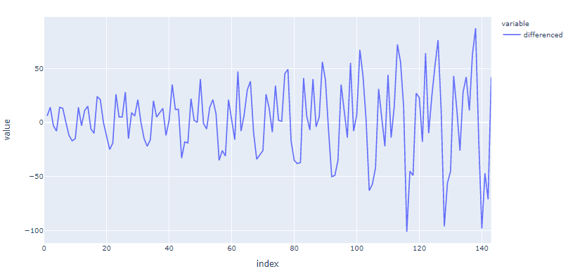

Differenced Time Series

The differenced time series appears to be stationary this time. We can again apply the Dickey-Fuller test to confirm the stationarity of the differenced time series.

ARIMA

Now that we have a stationary series, we can move ahead with our forecasting models. We will be using the ARIMA model, which stands for Auto-Regressive Integrative Moving Average for forecasting. It is a generalized version of the ARMA model and simply a combination of two distinct Auto-Regressive & Moving Average models.

Let’s understand it component-wise:

Auto-Regressive (AR(p))

An Auto-Regressive model predicts the value at the current timestamp using the regression equation made from values at previous timestamps. Only past data is used for predicting the value at the current timestamp. Series having autocorrelation indicates the requirement of the auto-regressive component in ARIMA.

Integrative (I(d))

This component helps in making the series stationary using the differencing. Differencing is simply an operation where an observation is subtracted from the observation at the previous time step. This operation makes the time series stationary (removes trend and seasonality components from time series). We have already applied it in the last step.

Moving Average (MA(q))

A Moving Average model uses the errors from past forecasts in a regression equation. This model assumes that the value at the current timestamp can be predicted using the errors from the past forecasts.

Integrate all these components to form the ARIMA equation:

Source: Towards Data Science

How do we find the p, d, q values?

While using an auto-ARIMA model, finding the optimum seasonal auto-regressive component(p), differencing component(d), and seasonal moving average component(q) is a lot easier. However, we are interested in manually determining these p, d, q components.

Following are some ways of determining the p, d, & q parameters of ARIMA:

• The autocorrelation plot helps determine the optimal set of q parameters for the Moving Average model.
• The partial autocorrelation plot helps determine the optimal set of p parameters for the Auto-Regressive model.
• An extended autocorrelation plot of the data confirms whether the combination of the AR and MA terms is required for forecasting.
• Akaike’s Information Criterion (AIC) assists in determining the optimal set of p, d, q. Usually, the model with a smaller absolute value of AIC is preferred.
• Schwartz Bayesian Information Criterion (BIC) is another alternative of AIC, and lower BIC is better for selecting the optimal p, d, q.

Finding the set of p and q values:

from statsmodels.graphics.tsaplots import plot_acf, plot_pacf
plot_acf(air_passengers["Passengers"].diff().dropna())

plot_pacf(air_passengers["Passengers"].diff().dropna())
plt.show()

For finding the AR component p, we need to look for a sharp initial drop in the partial autocorrelation plot. It is happening just after the first peak. So, the p component value can have either 1 or 2.

For finding the q value, we will need to see an exponential decrease in the autocorrelation plot. We are not looking for a drastic change; instead, we are looking for a curve settling down to saturation. We can see it is happening just after 1. So, q can also be taken as either 1 or 2.

Let’s implement ARIMA(1, 1, 1) model:

from statsmodels.tsa.arima.model import ARIMA

model = ARIMA(air_passengers['Passengers'].diff(), order=(1,1,1))
results_ARIMA = model.fit()

plt.plot(air_passengers['Passengers'].diff())
plt.plot(results_ARIMA.fittedvalues, color='red')
print('Plotting ARIMA model')
print(results_ARIMA.summary())

residuals = pd.DataFrame(results_ARIMA.resid)

residuals.plot(kind='kde')
plt.show()

Residuals mean is approximately centered around zero, AIC & BIC metrics indicate an okay-ish fit, and our ARIMA order is optimum, as per the ACF and PACF. But relying upon PACF and ACF for finding the optimum p and q often deceives to the true potential of the ARIMA model. We can always tweak parameters and see if they provide a good forecast for the problem instead of going with the conventional rules. Let’s try another combination:

model = ARIMA(air_passengers['Passengers'].diff(), order=(4,1,4))

results_ARIMA_updated = model.fit()
plt.plot(air_passengers['Passengers'].diff())

plt.plot(results_ARIMA_updated.fittedvalues, color='red')
print('Plotting ARIMA(4,1,4) model')
print(results_ARIMA_updated.summary())

residuals = pd.DataFrame(results_ARIMA_updated.resid)

residuals.plot(kind='kde')
plt.show()

ARIMA(4, 1, 4) is slightly better than ARIMA(1, 1, 1). Let’s also implement seasonal-ARIMA, which is the same as an ARIMA model, but it also considers the seasonality.

import statsmodels.api as sm

model=sm.tsa.statespace.SARIMAX(air_passengers['Passengers'],order=(7, 1, 7),seasonal_order=(1,1,1,12))
results=model.fit()

air_passengers['forecast']=results.predict(start=120,end=145)
air_passengers[['Passengers','forecast']].plot(figsize=(12,8))

Strengths & Limitations of ARIMA

Limitations:

• Forecasts are unreliable for an extended window
• Data needs to be univariate
• Data should be stationary
• Outliers are challenging to forecast
• Poor at predicting Turning Points

Strengths:

• Highly reliable Forecasts for a short window
• Short-run forecasts frequently outperform the results from complex models, but that also depends on data
• Easy to implement
• Unbiased Forecast
• Realistic Confidence Intervals
• High Interpretability

More Forecasting Models

• Exponential Smoothing
• Dynamic Linear Model
• Linear Regression
• Neural Network Models

Possible Interview Questions

Time series problems are quite famous and very useful across different industries. Interviewers ask questions on time series in two cases, 

• If we have written some project on time series in our resume.
• If the interviewer wants to hire you for the time series project.

Questions on this topic will be either generic, covered in this blog, or very specific to our projects. Possible questions on this topic can be:

1. What is time-series data, and what makes it different from other datasets?
2. What is a forecasting technique? Can you name some popular applications of it?
3. Why do we need to decompose the time-series dataset, and what are the possible ways?
4. What does the stationary test signify in time-series datasets?
5. What is the ARIMA model, and what do we do to find the value of parameters involved in this algorithm?

Conclusion

In this article, we discussed the essential details about the time series data and forecasting models. We played with the real-world data of Gold price, in which we learned stationary testing, log transformation, and data decomposition techniques. After that, we built and evaluated our ARIMA model on that. We hope you enjoyed the article.

Enjoy Learning! Enjoy Algorithms!