Divide and Conquer Algorithm

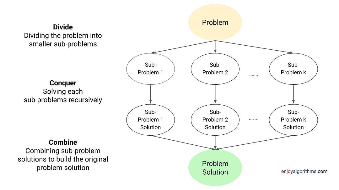
In data structures and algorithms, Divide and Conquer is a recursive problem-solving approach that divides the problem into smaller subproblems, recursively solves each subproblem, and combines the subproblem's solutions to get the solution of the original problem. So, there are four steps in the divide and conquer algorithm:

1. Divide Step: We divide the problem into one or more than one smaller subproblems. Here subproblems are the smaller versions of the same problem for smaller input sizes.
2. Conquer Step: We solve each subproblem recursively by calling the same function. Here recursion will automatically handle the work for us.
3. Combine Step: We combine the solutions of the subproblems to build the solution of the original problem. For this, we perform some additional operations other than recursive calls. Note: In some algorithms, this part is optional.
4. Base Case: This represents the smallest version of the problem where recursion will terminate and directly return the solution.

Note: Before learning this strategy, we recommend exploring the concept of recursion.

Critical ideas to implement divide and conquer algorithm

1. There can be multiple smaller subproblems of a problem. So we need to choose the correct subproblems to find the solution. In most situations, we divide the problem into two equal size subproblems.
2. We solve each subproblem recursively. So we need to carefully determine the input parameters for the recursive call of each subproblem.
3. The correct base case is crucial for the correctness of the divide and conquer algorithm. So we need to carefully identify the smallest version of the problem.
4. To implement the combine step, we must identify the correct operation for combining the solutions of subproblems. In most cases, the cost of these operations can be O(1), O(log n), O(n), or O(n^2).

Divide and conquer using one subproblem (Decrease and conquer)

Binary search algorithm

Based on a comparison with the middle value, we recursively search for the target value in either the left or right half. This process will continue until we find the target value or reach the base case. In other words, we solve the searching problem of size n using one sub-problem of size of n/2.

Divide: Calculate the mid index, i.e., mid = l + (r - l)/2.

Conquer

• If (X[mid] == key), return mid.
• If (X[mid] > key), recursively search the key in the left half. 
• If (X[mid] < key), recursively search the key in the right half.

Combine: There is no need for this step. Think!

Base case: When left end crosses the right end, the subarray size will be zero i.e. if (l > r), return -1.

Quick-select algorithm of finding kth smallest

Divide: We divide the array into two subarray using the partition algorithm (partition process similar to quick sort). After the partition, partition algorithm will return the index of the pivot. So array X[l, r] will look like this: X[l, pos - 1] < pivot < X[pos + 1, r]. Note: Here pos is the index of pivot after the partition.

Conquer: If pivot is present at index pos, then (pos - l) elements are smaller than the pivot. In other words, pivot is the (pos - l + 1)th smallest element in the array.

• If (pos - l + 1 == k), return X[pos].
• If (pos - l + 1 > k), recursively search kth smallest in the left subarray.
• If (pos - l + 1 < k), recursively search (k - (pos - l + 1))th smallest in the right subarray.

Combine: One of the sub-problems in the conquer step will return the value of the kth smallest. So there is no need to combine the sub-problems. Note: Assume that l <= k <= r.

Base case: If l == r, return X[l]. In other words, the case of a single-element is the base case.

Similar problems to explore 

• Recursive algorithm of searching an element in a BST
• Recursive solution of calculating power function
• Euclidean algorithm of finding GCD of two numbers
• Median of two sorted arrays of the same size

Divide and conquer using two sub-problems

Merge sort algorithm

We divide the array of size n into two equal sub-arrays of size n/2, recursively sort both sub-arrays and merge the sorted halves to sort the complete array.

• Divide: Calculate the mid index, i.e., mid = l + (r - l)/2.
• Conquer: Recursively sort both smaller halves.
• Combine: Merge both sorted halves to sort the whole array.
• Base case: When l == r, the sub-array has one element left, which is trivially sorted.

Quicksort algorithm

We divide the array into two sub-arrays using the partition algorithm and sort each sub-array recursively to get the final sorted array.

• Divide: Divide the problem into two smaller sub-problems by partitioning the array around the pivot. Here partition process will return the index of the pivot element.
• Conquer: Recursively sort both subproblems.
• Combine: This is a trivial case because our whole array will get sorted after sorting both smaller arrays.
• Base case: When l ≥ r, the sub-array will be either empty or one value left.

Divide and conquer solution of finding max and min

• Divide: Divide the array into two equal parts around the mid-value.
• Conquer: Recursively find the min and max of both left and right parts.
• Combine: Compare max and min of both halves to get the max and min of the whole array.
• Base case: If the subarray size is 1, return that single element as both max and min. If the subarray size is 2, compare both elements and return the max and min among them.

Divide and conquer solution of finding max subarray sum

We divide the array into two equal subarrays: X[l, mid] and X [mid + 1, r]. Then the sub-array X[i, j] with maximum sum must lie in one of these places: 1) Entirely in the left sub-array 2) Entirely in the right sub-array 3) Subarray crossing the mid-point.

• Divide: Calculate the mid index i.e., mid = l + (r - l)/2.
• Conquer: Recursively find the max sub-array sum of left and right halves.
• Combine: Calculate the maximum sub-array that crosses the mid-point and takes the maximum of all three possibilities.
• Base case: When l == r, there is only one element in the array, and we can directly return the max subarray sum as X[l] or X[r].

Divide and conquer solution of finding majority element

• Divide: Calculate the mid index, i.e., mid = l + (r - l) / 2.
• Conquer: Recursively find the majority element of the left and right halves.
• Combine: If the majority elements of the left and right halves are equal, then it will be the overall majority element. Otherwise, we count the frequency of the left majority and right majority in the array and return the maximum of them as an output.
• Base case: This is the case of a single-element array, i.e., if (l == r), return X[l] or X[r].

Similar problems to explore

• Divide and conquer solution of finding the max difference
• Finding the closest pair of points
• Building segment tree for range query operations
• Divide and conquer solution of the convex hull
• Divide and conquer solution of merging k sorted list
• Constructing binary tree from preorder and inorder
• Converting a sorted array to a balanced BST
• Divide and conquer solution of fast Fourier transform

Divide and conquer using more than two sub-problem

There are a few cases where we use more than two subproblems to get the solution to the final problem. We will add detailed insights about this idea later.

• Karatsuba algorithm of integer multiplication 
• Strassen matrix multiplication

Time complexity analysis of divide and conquer algorithm

We use recurrence relation to define the time complexity of divide and conquer algorithms. If T(n) is the time complexity for input size n, then T(n) = Time complexity of the divide part + Time complexity of the conquer part + Time complexity of the combine part.

• The time complexity of the divide part is O(1) in most of the scenarios because it calculates the middle index. However, there are a few exceptions! For example, the quicksort divide part is a partition process, which requires O(n) operations.
• Suppose we divide the problem into k number of different sub-problems and solve each sub-problem recursively. So, the time complexity of the conquer part = T(Input size of subproblem 1) + T(Input size of subproblem 2) + …. + T(Input size of subproblem k).
• The time complexity of the combine part depends on the cost of extra operations to combine the solution of smaller sub-problems. It can be O(1), O(n), O(n^2), etc., based on the nature of the operation.

The above approach provides a way to define the recurrence relation of the divide and conquer algorithm. Now we solve the recurrence relation and calculate the overall time complexity in terms of Big-O notation.

There are three popular ways to solve such recurrence relations: Recursion tree method, Master method and substitution method. You can explore this blog to understand the detailed analysis of divide and conquer algorithms: Analysis of recursion in programming.

Space complexity analysis of divide and conquer algorithm

We implement a divide and conquer algorithm using recursion, which involves a call stack. So the space complexity depends on the size of the recursion call stack, which is equal to the depth of the recursion tree. The overall space complexity of the divide and conquer algorithm = Size of recursion call stack + Extra space used inside the code.

It is essential to ensure that the memory allocated for the recursion stack is sufficient. Otherwise, the execution may fail due to stack overflow. In other words, time-efficient divide and conquer algorithms usually have a relatively small recursion depth.

Parallelism in divide and conquer algorithms

Since the sub-problems are independent, we can calculate them in parallel. In other words, divide and conquer is a natural parallel algorithmic approach that leads to a large amount of parallelism. Even if we only divide the problem into two sub-problems, each sub-problem will generate two more smaller sub-problems, and so on.

Because of this property, we can use divide-and-conquer algorithms for execution in multi-processor or shared-memory systems. There is no need to plan the data communication between processors in advance because we can execute distinct sub-problems on different processors.

Additionally, divide-and-conquer algorithms can make efficient use of memory caches. The idea is simple: Once a sub-problem is small enough, it can be solved within the cache without accessing the main memory.

Optimizing divide and conquer algorithms

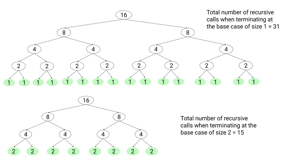
Sometimes, recursion with small base cases can lead to many recursive calls and huge recursive stacks. This may increase time and space complexity. On the other hand, we can choose the base case wisely to terminate recursion after fewer steps. This will reduce the number of recursive calls significantly and improve the performance.

For example, a quicksort algorithm could stop when there is a single input or input is empty. To improve efficiency, we can switch to a simple loop-based insertion sort algorithm once the number of items to be sorted is small enough. The idea is simple: Base case larger than two can reduce many recursive calls and the recursion stack size.

The following recursion tree diagram is an example of finding the maximum and minimum for an input size of 16 elements. We can observe that the total number of recursive calls will decrease if we terminate at a larger base case.

Sometimes, we can optimize the divide and conquer solution by reducing the total number of sub-problems. The idea is simple: it reduces the number of recursive calls significantly. The best examples of this are calculating the power function, Karatsuba algorithm, and Strassen matrix multiplication. We will provide more insights about this idea later in a separate blog.

Critical ideas to think in divide and conquer algorithm

• We can implement divide-and-conquer algorithms iteratively using an explicit stack or without using a stack. We recommend exploring the iterative implementation of binary search, merge sort and quicksort.
• We can reduce the risk of stack overflow by minimizing the parameters of the recursive calls.
• Using the divide and conquer approach, we can solve several challenging problems with less time complexity than their brute-force solutions. But to be efficient, one must ensure that the divide and combine steps are efficient.
• There is a difference between the recursive solution of divide and conquer and dynamic programming problems. Understanding this difference is important for mastering the dynamic programming approach. Explore this blog: Difference between dynamic programming and divide and conquer approach.
• We can solve several coding problems using the divide and conquer idea of binary search and merge sort.

We will keep updating this blog to add more insights. Please share your feedback or insights to improve this further. Enjoy learning, Enjoy algorithms!