Quick Sort Algorithm

Difficulty: Medium, Asked-in: Google, Microsoft, Adobe, Goldman Sachs, Qualcomm.

Quick sort algorithm was developed by computer scientist Tony Hoare in 1959.

Why quick sort important?

Quick sort is one of the fastest sorting algorithms, based on the idea of divide-and-conquer. There can be several reasons to learn quick sort:

• Often the best choice for sorting because it operates efficiently in O(n log n) on average.
• An excellent algorithm for understanding the concept of recursion. The recursive structure, flow of recursion, and base case are intuitive.
• One of the best algorithms for learning worst-case, best-case, and average-case analysis.
• The partition algorithm used in quick sort is based on the two-pointer approach, which can be applied to solve various coding questions.
• Quick sort is cache-friendly due to its in-place sorting property and reduced memory accesses.
• An excellent algorithm for exploring the concept of randomized algorithms.

Quick sort intuition

Suppose we partition an unsorted array around some input value (pivot) into two parts such that values in the left part are less than the pivot and values in the right part are greater than the pivot.

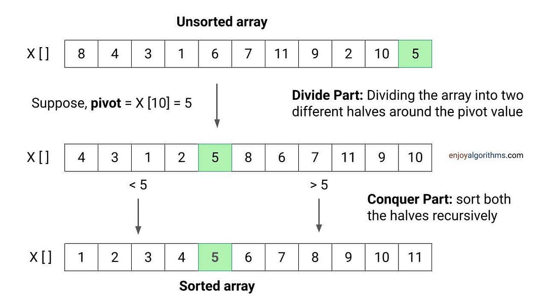
If we observe, the pivot will get placed in the correct position in the sorted output after the partition. This situation is similar to that of a sorted array, with one major difference: the left and right halves are still unsorted! If we observe further, both unsorted halves form smaller subproblems of the sorting problem.

So, if we sort both halves recursively, using the same function, the entire array will get sorted! The idea is simple: All values on the left side are less than the pivot, the pivot is at the correct position, and all values on the right side are greater than the pivot.

Divide and conquer idea of quick sort

The above idea of quicksort is the divide-and-conquer approach to problem-solving. Here we divide the sorting problem into two smaller subproblems using the partition algorithm and solve each subproblem recursively to get the final sorted array. We repeat the same process for smaller subarrays until we reach the base case.

Divide Part: Divide the problem into two smaller subproblems by partitioning the array X[l...r]. The partition process will return the pivotIndex i.e. the index of the pivot after the partition.

• Subproblem 1: Sort array X[] from l to pivotIndex - 1.
• Subproblem 2: Sort array X[] from pivotIndex + 1 to r.

Conquer Part: Sort both subarrays recursively.

Combine Part: This is a trivial case because after sorting both smaller arrays, the entire array will be sorted. In other words, there is no need for the combine part.

Quick sort implementation

Suppose we use the function quickSort(int X[], int l, int r) to sort the entire array, where l and r are the left and right ends. The initial function call will be quickSort(X, 0, n - 1).

Divide part

We define the partition(X, l, r) function to divide the array around the pivot and return the pivotIndex. We will select the pivot value inside the partition function. The critical question is: Why are we choosing the pivot value inside the partition function? Think and explore!

pivotIndex = partition(X, l, r)

Conquer part

• We recursively sort the left subarray by calling the same function i.e., quickSort(X, l, pivotIndex - 1).
• We recursively sort the right subarray by calling the same function i.e., quickSort(X, pivotIndex + 1, r).

Base case

Base case is the smallest version of the problem where recursion will terminate. So, in the case of quick sort, the base case occurs when the sub-array size is either 0 (empty) or 1. In other words, l >= r is the condition for the base case. The critical question is: When do we reach the empty subarray scenario? Think and explore!

Quick sort pseudocode

void quickSort(int X[], int l, int r)
{
    if (l < r)
    {
        int pivotIndex = partition(X, l, r)
        quickSort(X, l, pivotIndex - 1)
        quickSort(X, pivotIndex + 1, r)
    }
}

Quick sort partition algorithm

How can we divide an array around the pivot so that the values in the left part are less than the pivot, and values in the right part are greater than the pivot? Can we do it in place? Let’s think!

Suppose we choose the rightmost value as the pivot, i.e., pivot = X[r], and scan the array from left to right. Now we know that the starting part of the array should contain values less than the pivot. So whenever an element is less than the pivot, we will place it at the starting part of the array and move forward. Otherwise, we will ignore that element and move forward. How can we implement it? Let’s think!

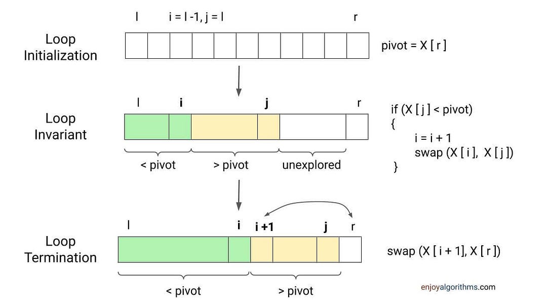
• We need two pointers: 1) Pointer i to track the starting subarray from 0 to i with values less than the pivot, and 2) Pointer j to traverse each element of the array.
• Now we scan the array from j = l to r - 1. If X[j] < pivot, we need to place the value X[j] at the starting part of the array at index i. So we increment pointer i, swap X[j] with X[i], and move forward. Otherwise If X[j] > pivot, we ignore the value at index j and continue to the next iteration.
• By the end of the loop, values in the subarray X[0 to i] will be less than the pivot, and values in the subarray X[i + 1 to r - 1] will be greater than the pivot.
• Now we place the pivot at its correct position, i.e., i + 1. For this, we swap X[r] with X[i + 1] and return the position of the pivot, i.e., i + 1.

Quick sort partition pseudocode

int partition (int X[], int l, int r)
{
    int pivot = X[r]  
    int i = l - 1
    for (int j = l; j < r; j = j + 1)
    {
        if (X[j] < pivot)
        {
            i = i + 1
            swap (X[i], X[j])
        }
    }
    swap (X[i + 1], X[r])
    return i + 1
}

Critical questions to think:

• Why did we initialize i with l - 1? Can we implement the code by initializing i with l?
• Does the above code work correctly when values are repeated?
• By the end of the loop, why is the correct position of the pivot i + 1?
• Can you think of implementing the partition process using some other idea?

Analysis of partition algorithm

We are running a single loop and doing constant operations at each iteration. In the worst or best case, we are doing one comparison at each iteration. So time complexity = O(n). We are using constant extra space, so space complexity = O(1). Note: Here swapping operation will depend on comparison if (X[j] < pivot).

Quick sort visualization

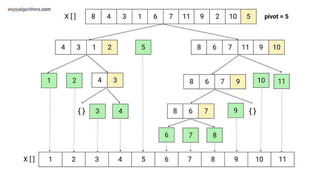
Quick sort time complexity analysis

Suppose T(n) is the worst-case time complexity of quick sort for input size n.

Now let's analyze it by breaking down the time complexities of each process:

• Divide part: Time complexity of the divide part = Time complexity of the partition = O(n).
• Conquer part: We are recursively solving two subproblems, where the size of the subproblems will depend on the choice of pivot in the partition. Suppose after the partition, i elements are in the left subarray and n - i - 1 elements are in the right subarray. So time complexity of the conquer part = Time complexity of sorting the left subarray + Time complexity of sorting the right subarray = T(i) + T(n - i - 1).
• Combine part: As mentioned above, this is a trivial part. Time complexity of combine part = O(1).

For calculating the time complexity T(n), we add time complexities of divide, conquer, and combine parts.

T(n) = O(n) + T(i) + T(n — i — 1) + O(1) 
= T(i) + T(n — i — 1) + O(n) 
= T(i) + T(n — i — 1) + cn

Recurrence relation of the quick sort
T(n) = c, if n = 1
T(n) = T(i) + T(n — i — 1) + cn, if n > 1

Worst-case analysis of quick sort

• The worst-case scenario will occur when the partition process always chooses the largest or smallest element as the pivot. In this case, the partition will be highly unbalanced, with one subarray containing n - 1 elements and the other subarray containing 0 elements.
• When we choose the rightmost element as the pivot, the worst-case will arise when array is already sorted in increasing or decreasing order. Here each recursive call will create an unbalanced partition.

For calculating the worst case time complexity, we put i = n  - 1 in the above formula of T(n).

T(n) = T(n - 1) + T(0) + cn 
T(n) = T(n - 1) + cn

Worst-case analysis of quick sort using Substitution Method

We simply expand the recurrence relation by substituting all intermediate value of T(i) (from i = n - 1 to 1). By end of this process, we ended up in a sum of arithmetic series.

T(n) 
= T(n - 1) + cn 
= T(n - 2) + c(n - 1) + cn
= T(n - 3) + c(n - 2) + c(n - 1) + cn
... and so on
= T(1) + 2c + 3c + ... + c(n - 2) + c(n - 1) + cn
= c + 2c + 3c + ... + c(n - 2) + c(n - 1) + cn
= c(1 + 2 + 3 + ... + n - 2 + n - 1 + n)
= c(n(n + 1)/2) 
= O(n^2)

Worst case time complexity of quick sort = O(n^2).

Worst-case analysis of quick sort using Recursion Tree Method

The recursion tree method is one of the popular techniques for recursion time complexity analysis. Here we draw a tree structure of recursive calls and highlight the extra cost associated with each recursive call. To get the overall time complexity, we add the cost level by level.

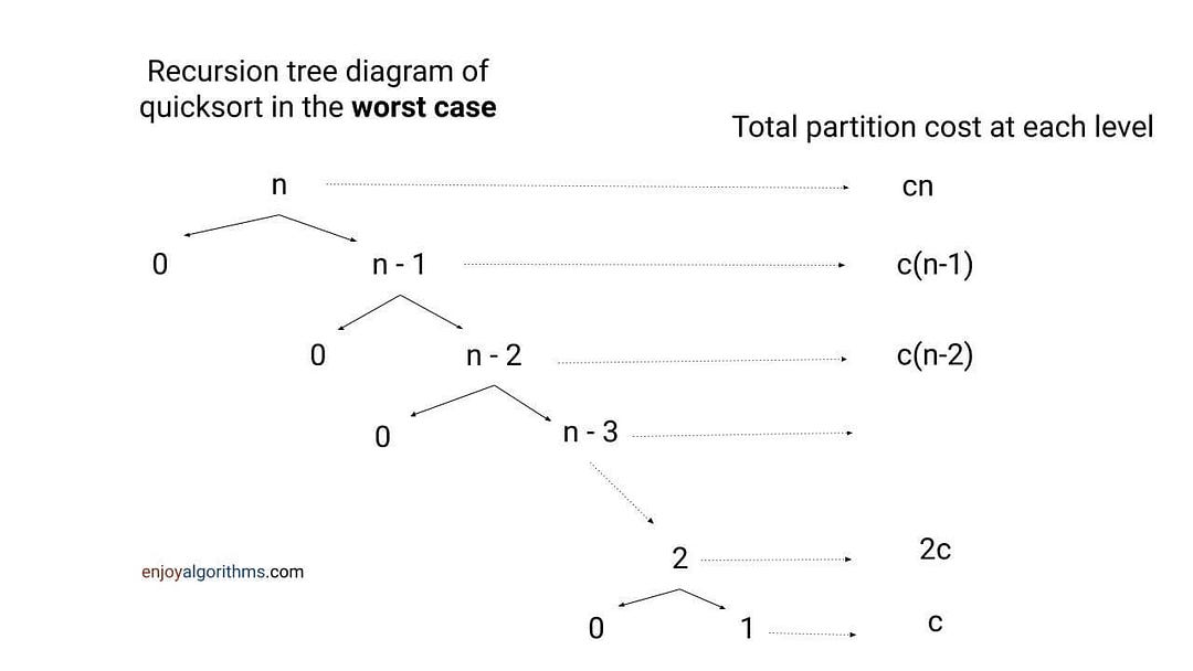
We sum the total partitioning cost for each level => cn + c(n−1) + c(n−2) +⋯+ 2c + c ​= c (n + n−1 + n−2 + ⋯+ 2 + 1) = c[n(n+1)/2] = O(n^2).

Best-case analysis of quick sort

The best-case scenario of quick sort will occur when partition process will always pick the median element as the pivot. In other words, this is a case of balanced partition, where both sub-arrays are approx. n/2 size each.

Suppose, the scenario of balanced partitioning will arise in each recursive call. Now, for calculating the time complexity in the best case, we put i = n/2 in the above formula of T(n).

T(n) = T(n/2) + T(n - 1 - n/2) + cn 
= T(n/2) + T(n/2 - 1) + cn 
~ 2 T(n/2)+ cn

T(n) = 2 T(n/2)+ cn

This recurrence is similar to the recurrence for merge sort, for which the solution is O(n log n). So the best-case time complexity of quick sort = O(n log n).

Average-case analysis of quick sort

Suppose all permutations of input are equally likely. Now, when we run the quick sort algorithm on random input, partitioning is highly unlikely to happen in the same way at each level of recursion. The idea is simple: The behaviour of quick sort will depend on the relative order of values in the input.

Here some of the splits will be reasonably well balanced and some of the splits will be pretty unbalanced. So the partition process will generate a mix of good (balanced partition) and bad (unbalanced partition) splits in the average case. These good and bad splits will be distributed randomly throughout the recursion tree. For a better understanding of the average scenario, suppose good and bad splits appear at alternate levels.

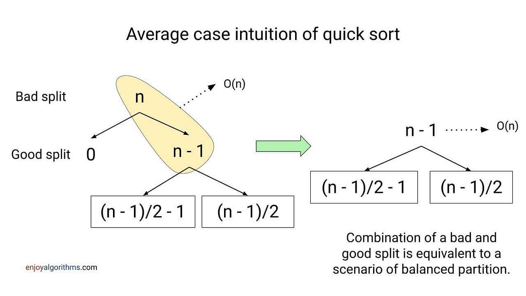
Suppose at the root, partition generates a good split, and at the next level, partition generates a bad split. The cost of the partition will be O(n) at both levels. So the combined cost of the bad split followed by the good split is O(n). Overall, this is equivalent to a single level of partitioning, which resembles the scenario of a balanced partition.

As a result, the height of recursion tree will be O(log n), and the combined cost of each level will be O(n). This is similar to the situation of the best case. So the average-case time complexity of quick sort will be O(n log n). 

Note: Average case time complexity is the same as the best case, but the value of the constant factor in O(n log n) will be slightly higher in the average case. 

For better visualization, let’s assume that the partition always produces a partially unbalanced split in the ratio of 9 to 1. The recurrence relation for this: T(n) = T(9n/10) + T(n/10) + cn. Image source: CLRS Book.

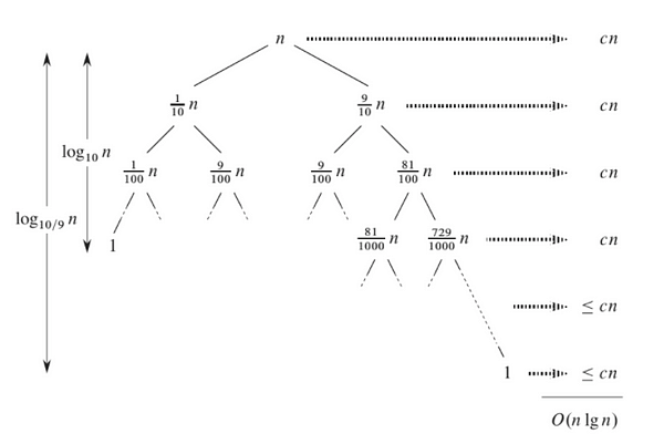
We can notice following things from above diagram:

• Left subtree is decreasing fast with a factor of 1/10. So the depth of left subtree = log10(n). Similarly, right subtree is decreasing slowly with a factor of 9/10. So the depth of right subtree = log10/9(n). Note: We can write log10/9(n) as O(logn). So the maximum depth of the recursion tree is still O(logn).
• At each level of recursion, the cost of partition is at most cn. After doing the sum of cost at each level, quick sort time complexity for such unbalanced split = cn*O(logn) = O(nlogn).
• With 9-to-1 proportional split at each level of recursion (which intuitively seems unbalanced), quick sort runs in O(nlogn) time. Even a 99-to-1 split can produce O(nlogn) time complexity!
• In general, any split of constant proportionality produces a recursion tree of depth O(logn), where cost at each level is O(n). So time complexity is O(nlogn) for any such type of split.

Quick sort apace complexity analysis

Quicksort is an in-place sorting algorithm because it does not use extra space in the code. However, every recursive program uses a call stack in the background. So the space complexity of quicksort will depend on the size of the recursion call stack, which will be equal to the height of the recursion tree. As mentioned in the above analysis, the height of the recursion tree depends on the partition process.

In the worst-case scenario, the partition will be unbalanced. So there will be only one recursive call at each level of recursion. In other words, the recursion tree will be skewed in nature, and its height will be O(n). So recursion will require a call stack of size O(n) and the worst-case space complexity of quick sort = O(n).

In the best-case scenario, the partition will be balanced. So there will be two recursive calls at each level of recursion. In such a scenario, the recursion tree will be balanced in nature. So, the height of the recursion tree = O(log n), and recursion will require a call stack of size O(log n).

Case of repeated elements in quick sort algorithm

In the above algorithm, we assume that all input values are distinct. How do we modify quick sort algorithm when input values are repeated? Let’s think!

We can modify the partition algorithm and separate input values into three groups: Values less than pivot, values equal to pivot and values greater than pivot. Values equal to pivot are already sorted, so only less-than and greater-than partitions need to be recursively sorted. Because of this, we will return two index startIndex and endIndex in the modified partition algorithm.

• Elements from l to startIndex - 1 are less than pivot.
• Elements from startIndex to endIndex are equal to pivot.
• Elements from endIndex + 1 to r are greater than pivot.

Modified pseudocode for repeated elements

void quickSort(X[], l, r)
{
    if (l < r)
    {
        [leftIndex, rightIndex] = partition(X, l, r)
        quickSort(X, l, leftIndex - 1)
        quickSort(X, rightIndex + 1, r)
    }
}

Critical question: How can we implement the partition algorithm for this idea?

Strategy to choose pivot in quick sort partition algorithm

As we know from the analysis, the efficiency of quick sort depends on the smart selection of the pivot. So there can be many ways to choose the pivot:

• Choosing the last element as the pivot.
• Choosing the first element as the pivot.
• Selecting a random element as the pivot.
• Selecting the median as the pivot.

In the above implementation, we have chosen the rightmost element as the pivot. This can result in a worst-case situation when the input array is sorted. The best idea would be to choose a random pivot that minimizes the chances of a worst-case at each level of recursion. Selecting the median element as the pivot can also be acceptable in the majority of cases.

Pseudocode for median-of-three pivot selection

mid = l + (r - l)/ 2

if X[mid] < X[l]
    swap (X[l], X[mid])

if X[r] < X[l]
    swap (X[l], X[r])

if X[mid] < X[r]
    swap (X[mid], X[r])

pivot = X[r]

Critical ideas to think!

• Quick sort is an unstable sorting algorithm i.e. the relative order of equal elements might not be preserved after sorting. So how can we modify the quick sort algorithm to make it stable?
• Quicksort is an in-place sorting algorithm where we use extra space only for recursion call stack but not for manipulating input. So what would be the average case space complexity of quick sort? How can we optimize space complexity to O(logn) in the worst case?
• How can we implement quick sort iteratively using a stack?
• When do we prefer quick sort over merge sort for sorting arrays?
• How can we sort linked list using quick sort? Why we prefer merge sort over quick sort for linked lists?
• BST sort or tree sort is also similar to the Quick sort, where both algorithms make the exact number of comparisons but in a different order.
• We can use a quick sort partitioning process to efficiently find the kth smallest element or largest element in an unsorted array. This problem is called Quick-Select, which works in O(n) time on average.

Concepts to explore further

• The idea of Hoare partition
• Quicksort optimization using tail recursion approach

Coding problems to explore (similar to partition)

• Dutch national flag problem
• Move all zeroes to end

Content references

• Algorithms by CLRS
• The Algorithm Design Manual by Steven Skiena

If you have any queries or feedback, please write us at contact@enjoyalgorithms.com. Enjoy learning, Enjoy coding, Enjoy algorithms!