AVL Tree Data Structure

A Binary Search Tree(BST) is a binary tree data structure, where each node has the following properties:

• The node's left subtree contains only nodes with keys smaller than or equal to the node's key.
• The node's right subtree only contains nodes with keys greater than the node's.
• The left and right subtrees are valid binary search trees.

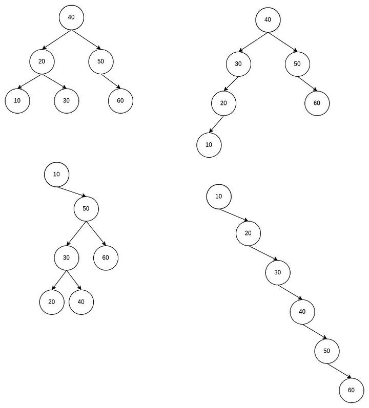
Following are some examples of binary search trees:

Why are binary search trees useful?

The primary use of binary search trees is for searching. Searching for a given value in a binary search tree is easy because elements in BST are stored in a sorted order i.e. the inorder traversal of a binary search tree gives the data in sorted order. Following are the steps for searching for a given element in a BST:

• Compare the element with the root of the tree.
• If the value is the same, then return the node.
• Otherwise, check if the given element is less than the root's value. If so, move to the left subtree. If not, move to the right sub-tree.
• Repeat the above process recursively or iteratively until the given element matches the root's value.
• If we reach a leaf node, and the element is not found, return false.

Let's see some examples of searching in a BST. Consider the top-left BST from the first image, and we want to search for the number 30. We start from the root. As the value of the root, 40, is greater than the 30, we move to the left child. The current node's value, 20, is less than 30, so we move to the right child. As the value of the current child is equal to 30, we have found the element we were searching for. Suppose we wanted to find 35 instead of 30; we would have followed the same path till node 30. As 30 is less than 35, we will move to the left child. However, the current node does not have a left child. This means 35 is not present in the tree.

As we can see from the above algorithm and examples, the time complexity of searching for a node in a BST depends on its height. The worst-case time complexity of searching for a node in the BST is O(n). This is the scenario of a skewed tree where each level has only one node and the height of the tree is n (Here n is the number of nodes in the BST). The best-case time complexity of searching in a BST is O(logn), as the minimum height achieved for a binary tree with n nodes is logn. Such a type of BST is known as a balanced binary search tree.

Let's see an example where the time complexity of searching in a BST is not optimal. Consider the bottom right BST from the first image. Suppose we want to search for 60 in the BST. We must traverse all six nodes, equivalent to a linear search.

Why is there a difference in the search times in the two BSTs, even though they have the same set of nodes? Because their structure is different. Even though both BSTs have the same set of nodes, their structure depends on the insertion order of the nodes into the BST. This is the drawback of BSTs. The time required for searching for a given element varies from O(logn) to O(n), depending on the insertion order. Can we improve this?

Introduction to AVL Tree Data structure 

AVL Trees, named after its inventors Adelson-Velsky and Landis, is a unique variation of the Binary Search Tree, which is a self-balancing BST. The property of AVL Trees is that they automatically attain the tree's minimum possible height after executing any operation.

We have the following three elements,{10, 20, 30}, and we want to insert them into a BST. There are 6(3!) ways of inserting the values into the BST. The following image shows the different orders and the resulting BSTs.

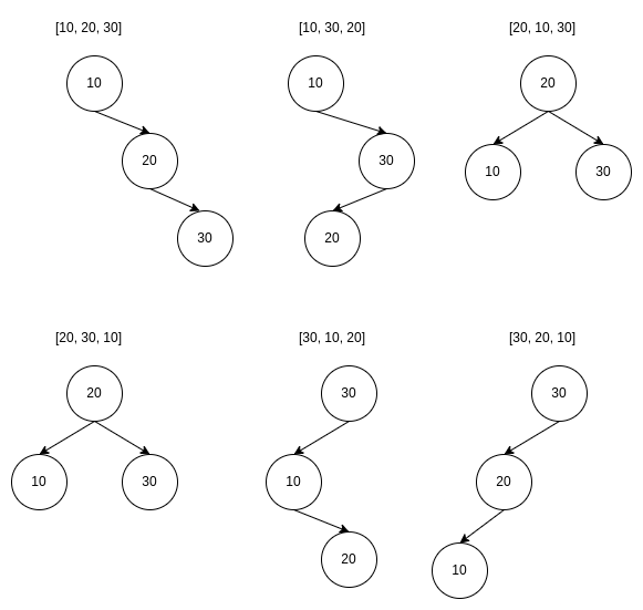
Two orders result in a BST of height 1, whereas the remaining four result in height 2. Try to think if there is any way of converting the height 2 BSTs into height 1 BSTs. We can do some rotations while maintaining the BST property to convert the BSTs of height 2 into a BST of height 1.

Balance Factor

We define a term balance factor for each node. The balance factor for a node is the difference between the height of its left subtree and right subtree. Balance factor = abs(height of right subtree — height of the left subtree).

In an AVL tree, all nodes should have a balance factor in {0, 1}. The following image shows the balance factor for each node for all BSTs from the first image. The value in red is the balance factor of each node.

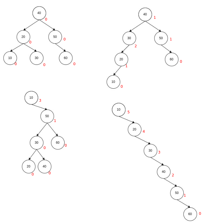
We can also follow the other convention, where we just take the difference between the height of the left subtree and the height of the right subtree. Here negative balance factor indicates right imbalance, positive balance factor indicates left imbalance.

int get_balance_factor(Node * node)
{
    if(node == NULL)
        return 0;
    // balance factor = left subtree height - right subtree height
    return (get_height(node->left) - get_height(node->right));
}

All Types of Possible Rotations

As we had seen earlier, if a BST is not balanced, rotations are required to convert that tree to a balanced BST(AVL Tree). Let's study each type of rotation in detail.

LL Rotation
Consider the following insertion order:

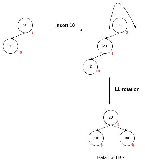
We can see that initially, the tree was balanced. However, after the insertion of 10, the tree became imbalanced. Node 10 was inserted to the left of the left of the root node. Thus, this type of imbalance is a left-of-left imbalance. This imbalance indicates that the tree is heavy on the left side. Therefore, a right rotation is applied to counter the left imbalance, and the tree becomes a balanced tree. This rotation can be visualized as pulling a rope around a nail to balance it, so it does not fall off the nail.

Node * LL_rotation(Node * node)
{
    Node * child = node->left;
    node->left = child->right;
    child->right = node;
    node->height = max(get_height(node->left),
                        get_height(node->right)) + 1;
    child->height = max(get_height(child->left),
                       get_height(child->right)) + 1;
    return child;
}

RR Rotation
This case is similar to LL Rotation, but the tree gets unbalanced after the insertion of a node into the right subtree of the right child of the imbalance node. This type of imbalance is known as a right-of-right imbalance. 
Consider the following insertion order to understand this scenario:

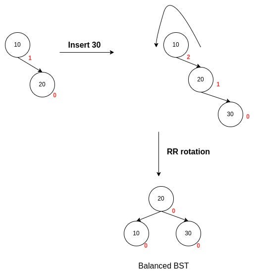
The tree became heavy on the right, and a left rotation can be performed to counter the right imbalance.

Node * RR_rotation(Node * node)
{
    Node * child = node->right;
    node->right = child->left;
    child->left = node;
    node->height = max(get_height(node->left),
                         get_height(node->right)) + 1;
    child->height = max(get_height(child->left),
                        get_height(child->right)) + 1;
    return child;
}

LR Rotation

So far, we saw cases where the imbalance was in one direction only(LL or RR). However, as shown in the image, the imbalance is on the right of the left node. Try to see that it is impossible to balance the tree in a single rotation. Let's see how to balance this tree.

Consider the following insertion order:

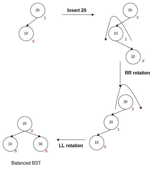
As we can see, after applying a left rotation on the left node of the root node, we get a left-of-left imbalance. We have seen how to handle this case; we perform a right rotation on the root. Now, the tree becomes balanced. So, the right-of-left imbalance can be corrected by an LR rotation. Steps of LR rotation:

1. Perform a left rotation on the left subtree of the imbalanced node as the left child has a right imbalance. This process turns the imbalance from right-of-left to left-of-left.
2. Perform a right rotation on the imbalanced node to balance the left imbalance.

RL Rotation
RL rotation is similar to LR rotation; it is done when the tree gets unbalanced upon insertion of a node into the left subtree of the right child of the imbalance node right-of-left insertion. Consider the following insertion order to understand this scenario:

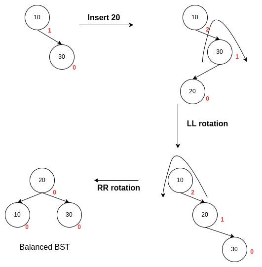
We can see that the parent of the inserted node becomes imbalanced on the left, so a right rotation should be performed on the parent of the inserted node to convert the tree into a right-of-right imbalance. We have seen earlier that a left rotation should be performed to remove the right-of-right imbalance.

We have seen different types of operations which can remove the imbalance in an unbalanced BST. While making rotations in a big tree, note that, as discussed, always focus on three nodes and balance them step by step. Multiple nodes can get imbalanced after inserting or deleting a node from an AVL Tree. We have to take care to keep the entire tree balanced after any operation. We need to traverse the ancestors of the inserted/deleted node in the tree and perform rotations on the first occurred imbalanced node. We need to continue this process until the whole tree is balanced. This process of rebalancing from the bottom to the top of the tree is discussed in the following section.

Operations on the AVL Tree

Insertion in AVL tree

Before studying insertion in AVL trees, let's briefly recap insertion in BSTs. We traverse the tree from the root using the BST logic to insert a new node in a BST. Following is the BST logic:

1. If the value of the current node is less than the value of the node to be inserted, we move to the left child of the current node.
2. Else, if the value of the current node is greater than the value of the node to be inserted, we move to the right child of the current node.
3. Otherwise, if the current node's value equals the value inserted, we return as we maintain nodes with unique values in the BST.

We traverse the tree till the leaf node of the BST. Then we insert the node in the correct position(left or right, depending on the BST logic).

Similar to the insertion in BSTs, the new node is inserted as a leaf node in AVL Trees. The balance factor of the new node inserted as a leaf node always equals 0. The insertion of this new node in the tree may change the balance factor of other nodes in the tree. We have to check if the tree is balanced or not. To do the same, we have to check the balance factor of only the ancestors. Try to think why we need to check only the ancestors' balance factor and not the balance factor tree's other nodes.

When we insert a new node in a tree, only the ancestors' height is altered, creating an imbalance as their balance factor might change. So we traverse from the image parent of the inserted node to the top of the tree, fixing any imbalances in the way. This process of finding imbalances by traversing the ancestors of the newly inserted node is known as retracing. If the tree becomes unbalanced after inserting a new node, retracing helps us find the nodes in the tree at which we need to perform the tree rotations to balance the tree.

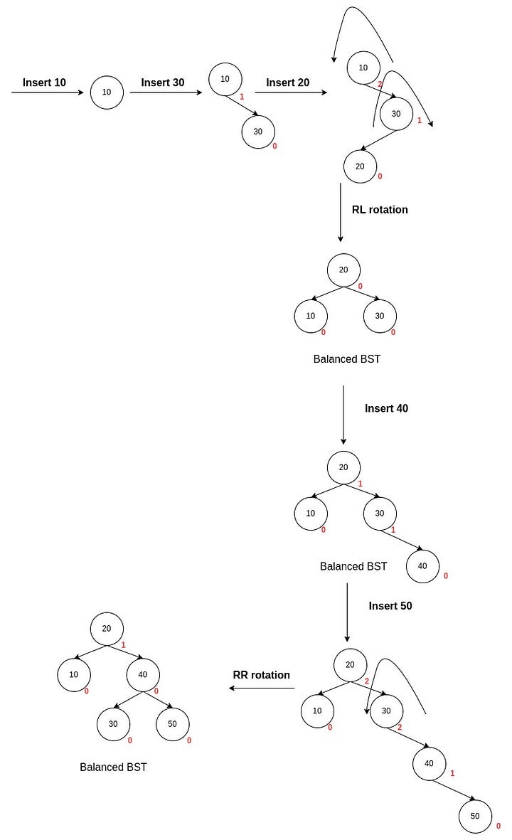
Let's summarise the steps for inserting a node in an AVL tree.

1. Insert the node in the tree using BST insertion logic.
2. Calculate and check the balance factor of each node which is an ancestor of the inserted node.
3. Perform tree rotations if required according to the type of imbalance.
4. Retrace till the root node.

AVL tree insertion java code

Node * insert(Node * node, int val)
{
    if(node == NULL)
    {
        // inserting as a leaf node
        node = new Node;
        node->data = val;
        node->left = NULL;node->right = NULL;
        node->height = 0;
        return node;
    }

    // BST logic 
    if(node->data < val)
        node->right = insert(node->right, val);
    else
        node->left = insert(node->left, val);

    // Update Height
    node->height = max(get_height(node->left), get_height(node->right)) + 1;
    // Get Balance factor
    int b = get_balance_factor(node);

    // Left heavy 
    if(b > 1)
    {
        // LL Rotation 
        if(get_balance_factor(node->left) == 1)
            node = LL_rotation(node);
        // LR Rotation
        else
        {
            node->left = RR_rotation(node->left);
            node = LL_rotation(node);
        }
    }
    // Right Heavy
    else if(b < -1)
    {
        // RR Rotation Case
        if(get_balance_factor(node->right) == -1)
            node = RR_rotation(node);
        // RL Rotation
        else
        {
            node->right = LL_rotation(node->right);
            node = RR_rotation(node);
        }
    }
    return node;
}

Time complexity analysis of insertion in AVL Trees

There are three main steps in insertion: searching where the node will be inserted, inserting the node, and retracing while removing the imbalances.

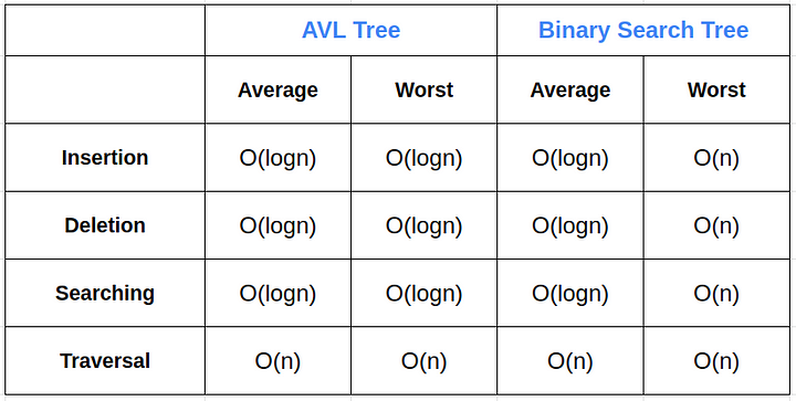
As the AVL Tree is balanced, searching where the node will be inserted by BST logic takes O(logn) time, as the tree's height will be logn if n nodes are present. This is a substantial improvement over the worst case in BST insertion as it takes O(n) time for searching in a BST. Inserting the node at the leaf takes O(1) time. Retracing takes O(logn) time; at each level of the tree at max, one node must be rebalanced, and rebalancing by rotation takes O(1) time by rotation at each node. Thus the overall time complexity of inserting a node in an AVL Tree is O(logn).

Deletion in AVL tree

Before studying deletion in AVL trees, let's briefly recap insertion in BSTs. We traverse the tree from the root using the BST logic to search for the node in a BST. If we reach the end(NULL node), the node to be deleted is not present in the tree.

Now, suppose the element is found in the tree. There are three different cases in which the deletion operation can be done depending upon the number of children of the node:

Case 1: When the node to be deleted is a leaf node: Then the node can be deleted directly as it does not have any children, i.e. it is a leaf node.

Case 2: When the node to be deleted has one subtree: In this case, the node to be deleted is replaced by its only child.

Case 3: When the node to be deleted has both the subtrees: This is a tricky case, as we need to decide with which node the node to be deleted has to be replaced. We can choose either a node from the left or right subtree.

If we choose a node from the left subtree, then the node should have the largest value in the left subtree to satisfy the BST property after replacing it with the node to be deleted.

If we choose a node from the right subtree, then the node should have the smallest value in the right subtree to satisfy the BST property after replacing it with the node to be deleted.

The deletion in AVL trees is just like BSTs, depending on the number of children of the node to be deleted. However, we need to verify that the tree remains balanced after deletion in an AVL tree, which is not the case in BST deletion. This can be done by balancing each node in the retracing process, as discussed in the insertion operation.

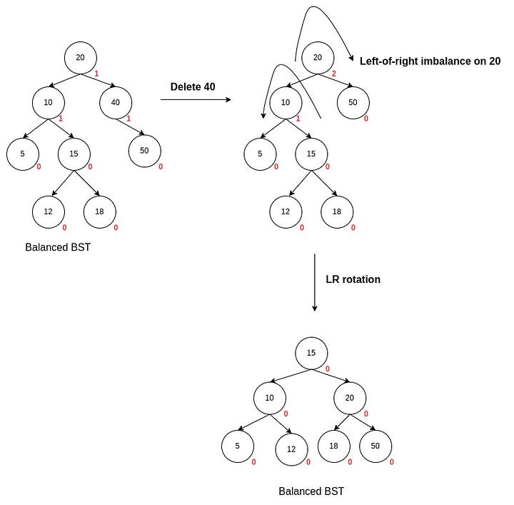
Let's summarise the steps for deleting a node in an AVL tree.

1. Search node in the tree by the BST logic. If the element is not present, return.
2. Delete the node.
3. While retracing, calculate and check the balance factor of each ancestor node.
4. Remove the imbalance using rotations.
5. Repeat from step 3 till the root of the tree.

AVL tree deletion java code

Node * deleteNode(Node * node, int val)
{
    // val not found in tree
    if(node == NULL)
        return node;
        
    // BST logic 
    if(node->data < val)
        node->right = insert(node->right, val);
    else if(node->data > val)
        node->left = insert(node->left, val);
    else
    {
        // Case 1
        if( (node->left == NULL) || (node->right == NULL) )
        {
            Node *temp = root->left ? root->left : root->right;
            // Case 1: No child case
            if (temp == NULL)
            {
                temp = root;
                root = NULL;
            }
            // Case 2: One child case
            else
                *root = *temp;
            free(temp);
        }
        else
        {
            // Case 3: two children: Get smallest in the right subtree
            Node* temp = minValueNode(root->right);
            root->data = temp->data;
            root->right = deleteNode(root->right, temp->data);
        }
    }

    // Update Height
    node->height = max(get_height(node->left), get_height(node->right)) + 1;
    // Get Balance factor
    int b = get_balance_factor(node);
    // Left heavy 
    if(b > 1)
    {
        // LL Rotation 
        if(get_balance_factor(node->left) == 1)
            node = LL_rotation(node);
        // LR Rotation
        else
        {
            node->left = RR_rotation(node->left);
            node = LL_rotation(node);
        }
    }
    // Right Heavy
    else if(b < -1)
    {
        // RR Rotation Case
        if(get_balance_factor(node->right) == -1)
            node = RR_rotation(node);
        // RL Rotation
        else
        {
            node->right = LL_rotation(node->right);
            node = RR_rotation(node);
        }
    }
    return node;
}

Time complexity analysis of deletion in AVL Trees

Similar to insertion, there are three main steps: searching for the node to be deleted, deleting the node, and retracing while removing the imbalances.

As the AVL Tree is balanced, searching where the node will be inserted by BST logic takes O(logn) time, as the tree's height will be logn if n nodes are present. Deleting the node takes O(logn) time in the worst case, as we might need to go to the right-most or left-most nodes of the left and right subtree, respectively, if the node to be deleted has both children. Retracing takes O(logn) time; at each level of the tree at max, one node must be rebalanced, and rebalancing by rotation takes O(1) time by rotation at each node. Thus the overall time complexity of inserting a node in an AVL Tree is O(logn).

You can find the complete class-based Java implementation at this link: https://gist.github.com/PrasannaIITM/57a0548a9ed6edf31dfff19add2b4d90

Conclusion

AVL Tree improves the performance of BST in the worst case by maintaining its height to logn by performing tree rotations according to the balance factor of each node.

Enjoy learning, Enjoy algorithms!