Boston House Price Prediction Using Support Vector Regressor

The surrounding environment highly influences house prices. For instance, a house in Beverly Hills may cost you a mind-blowing 40,00,000 US Dollars. Notably, it is the home to all the famous Hollywood celebrities. On the contrary, a house in any secluded region may come at a low budget. Still, the area will be prone to crime, and standard services like the police stations, schools, grocery stores, etc., may not be available in the vicinity. There is a clear trade-off between the locality and price. Whenever we have an issue associated with an exchange, we can always use Machine Learning to find the optimal solution to the problem.

Key takeaways from this blog

After reading this blog, we would be able to answer the following questions:

1. Why do we need Machine Learning models to solve the problem of house price prediction?
2. What are the factors that affect house prices?
3. Which machine learning models can be used to predict house prices?
4. Possible interview questions on this project.

Following are the set of features that we will use to build the machine learning model to predict house prices.

• CRIM: Per capita crime rate by town
• ZN: Proportion of residential land zoned for lots over 25,000 sq. ft.
• INDUS: Proportion of non-retail business acres per town
• CHAS: Charles River dummy variable (1 if tract bounds river; 0 otherwise)
• NOX: Nitric oxides concentration (parts per 10 million) [parts/10M]
• RM: Average number of rooms per dwelling
• AGE: Proportion of owner-occupied units built before 1940
• DIS: Weighted distances to five Boston employment centers
• RAD: Index of accessibility to radial highways
• TAX: Full-value property-tax rate per $10,000 [$/10k]
• PT-RATIO: It is the Pupil-Teacher ratio by the town
• B: The result of the equation B=1000(Bk — 0.63)² where Bk is the proportion of blacks by town
• L-STAT: Percentage lower status of the population
• MEDV: Median value of owner-occupied homes in $1000s
• We can see that the input attributes have a mixture of units.

Probably in the future, you will consider all these factors before fixing a deal.

Data Analysis 

Our objective is to build a machine learning model to predict house prices. However, before diving into the prediction task, we want to perform some exploratory data analysis to gain a basic understanding of the house price data, followed by feature selection and engineering. We are going to use the Boston house price dataset on Kaggle for this analysis. MEDV (Median House Price) is our target variable which we want to predict using the given set of independent features.

Let’s take a look at the data:

import pandas as pd
house_price = pd.read_csv('boston.csv')
house_price.head()

House Price Data

Our dataset contains 13 independent features. Let’s see if we have some collinear features in the dataset. Such features are redundant and can be removed for ease of analysis. Let’s check the correlation:

import seaborn as sns
import matplotlib.pyplot as plt
plt.figure(figsize=(20, 10))
cmap = sns.diverging_palette(500, 10, as_cmap=True)
sns.heatmap(house_price.corr().abs(), cmap=cmap, center=0, square=True, annot =True)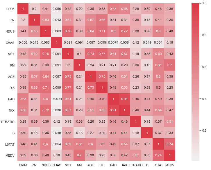

Correlation Matrix

From the above correlation matrix, we can see that TAX and RAD are highly correlated, and any one of them can be discarded. Also, LSTAT, RM, NOX, INDUS, PRTAIO, and TAX have a correlation greater than 0.4 with MEDV, which is a good indicator for using these parameters as predictors. Let’s visualize the relationship between these features vs. Median House Price (MEDV):

fig, axs = plt.subplots(nrows=2, ncols=4, figsize=(20,8))
cols = ['LSTAT', 'INDUS', 'NOX', 'PTRATIO', 'RM', 'TAX', 'DIS', 'AGE']
for col, ax in zip(cols, axs.flat):
    sns.regplot(x = house_price[col],y = house_price['MEDV'], color = 'red', ax=ax)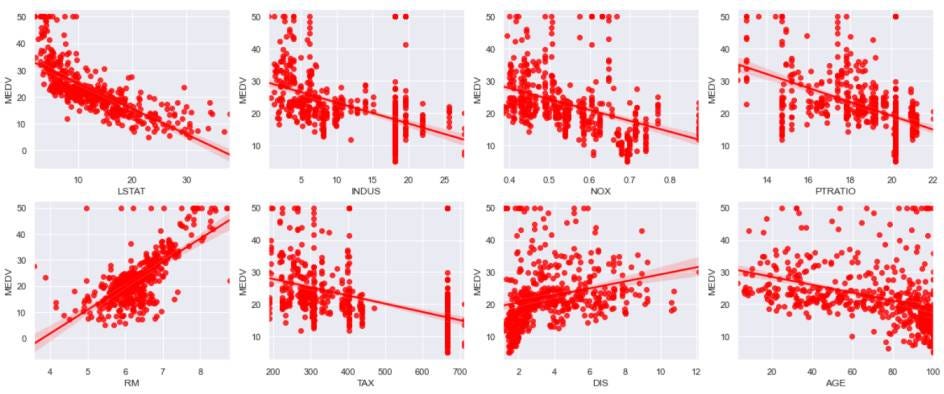

Scatter Plot

The majority of the features show a negative relationship to the house prices. Only a few features show a positive relationship. 

Let’s check the Boxplot for finding the outliers, if available:

fig, axs = plt.subplots(ncols=4, nrows=2, figsize=(10, 5))
index = 0
axs = axs.flatten()
for k,v in house_price.items():
    sns.boxplot(y=k, data=house_price, ax=axs[index])
    index += 1
plt.tight_layout(pad=0.4, w_pad=0.5, h_pad=5.0)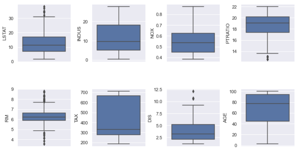

Boxplot

Only RM seems to have some significant outliers. Let’s remove them!

house_price = house_price[~((house_price['RM'] >= 8.5) | (house_price['RM'] < 4))]

Let’s summarize our data analysis steps:

• We used a correlation heatmap for finalizing the relevant set of features required for the analysis.
• Further, we visualized the relation of independent features to the target variable Median House Price using the reg-plot. We found a majority of attributes have a negative relationship with respect to the median house price.
• Finally, we used the Boxplots to confirm the presence of outliers in the dataset. However, we only found the outliers for RM (Average room) feature. In the subsequent step, we carefully removed the outliers.

Model Building 

We want to build a model which can take house-surrounding parameters as input and return an estimated price of the house based on the above discussed independent features. We will address this problem by building a regression model. This approach will eliminate a lot of manual visits, meetings with brokers & dealers, and paperwork required for estimating the price of a property. Companies like 99acres, MagicBricks, and Housing.com have already automated the house price estimation mechanism based on the surrounding parameters and housing requirements. We will be doing the same, but first, we need to select a regression model. 

This is a classic regression problem where we have the independent features as input and house price as the target. We need to select a supervised regression algorithm to accomplish this task. Let’s look at some regression algorithms that can be used for predicting the house price. 

• Linear Regression
• Decision Tree Regressor 
• Support Vector Regressor 
• K-NN Regressor 
• Random Forest Regressor 

Linear Models are relatively less complex and explainable, but linear models perform poorly on data containing the outliers. Also, linear models fail to perform well on non-linear datasets. In such cases, non-linear regression algorithms Random Forest Regressor and XGBoost Regressor perform better in fitting the non-linear data.

We don’t have significant outliers in our dataset, indicating that we can use linear as well as complex models. However, the model must have the following qualities:

• Simple & Explainable 
• Provides accurate predictions 
• Robust to concept drift and outliers
• Easy to deploy

We should always look for the above points in mind while selecting a regression model. For this tutorial, we will be using the Support Vector Regressor. 

Support Vector Regressor 

Support Vector Machine is a supervised machine learning algorithm that can be used for both classification and regression tasks. Support Vector Regression works on the same principle as that of an SVM. The important idea behind the SVR is to find the best-fit hyper-plane along with the optimum threshold. The optimum threshold value is the distance between the hyperplane and the boundary line. The boundary line is defined by the support vectors that lie farthest to the hyperplane. It is similar to fit the best fit line along with some threshold limits. The threshold limit is the distance between the hyperplane and the boundary line.

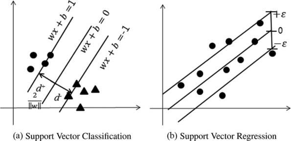
Source: ResearchGate

Following are some characteristics of SVR:

• SVR is sensitive to outliers (for Hard Margin only)
• Considers outermost data points for the determination of margin
• SVR is insensitive to inner data points 
• SVR can tackle non-linear data using the Kernel Trick

Let’s implement SVR to predict the house prices:

from sklearn.svm import SVR
from sklearn.preprocessing import MinMaxScaler
from sklearn.model_selection import train_test_split
target = house_price['MEDV']
features = house_price.drop('MEDV', axis = 1)
X_train, X_test, Y_train, Y_test = train_test_split(features, target, test_size=0.3)
scaler = MinMaxScaler(feature_range=(0, 1))
X_train = scaler.fit_transform(X_train)
X_train = pd.DataFrame(X_train)
X_test = scaler.fit_transform(X_test)
X_test = pd.DataFrame(X_test)
# Baseline SVR Model
regressor = SVR(kernel = 'rbf')
regressor.fit(X_train, Y_train)
regressor.score(X_test, Y_test)
# R-Squared Score: 0.705

Implementing SVR with Hyper-Parameter Tuning:

from sklearn.model_selection import GridSearchCV
from sklearn.metrics import mean_squared_error
from sklearn.metrics import make_scorer
K = 15
parameters = [{'kernel': ['rbf'], 'gamma': [1e-4, 1e-3, 0.01, 0.1, 0.2, 0.5, 0.6, 0.9],'C': [1, 10, 100, 1000, 10000]}]
print("Tuning hyper-parameters")
scorer = make_scorer(mean_squared_error, greater_is_better=False)
svr = GridSearchCV(SVR(epsilon = 0.01), parameters, cv = K, scoring=scorer)
svr.fit(X_train, Y_train)
print("Grid scores on training set:")
means = svr.cv_results_['mean_test_score']
stds = svr.cv_results_['std_test_score']
for mean, std, params in zip(means, stds, svr.cv_results_['params']):
    print("%0.3f (+/-%0.03f) for %r"% (mean, std * 2, params))

# Best parameters at C = 1000, gamma = 0.9, kernel = 'rbf'
regressor_tuned = SVR(kernel = 'rbf', C = 1000, gamma = 0.9)
regressor_tuned.fit(X_train, Y_train)
regressor_tuned.score(X_test, Y_test)
# R-Squared Score: 0.821
# 16.45 % Improvement in R Squared Score

After hyper-parameter tuning, the R-Squared score jumped from 0.70 (Baseline SVR model) to 0.82 (Hyper-tuned SVR model), which is a massive 16.45% overall improvement. 

Let’s visualize the residuals on the test and train set: 

plt.figure(figsize=(10,6))
visualizer = ResidualsPlot(regressor_tuned)
visualizer.fit(X_train, Y_train) 
visualizer.score(X_test, Y_test) 
visualizer.show();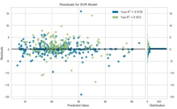

Residuals are centered around zero, which indicates a good fit. Also, the R-squared score indicates a reliable fit for predicting house prices.

Industrial Use Cases

99acres

99acres is an Indian Real Estate Property dealing company launched in 2005 for automating the Buy, Sell, rent business on properties. Over the years, it has gained the title of India’s number 1 property portal. 99acres uses regression modeling for the estimation of house valuations, rent, and land prices.  

Amazon 

Amazon is an American multinational tech company that focuses primarily on e-commerce and Artificial Intelligence. Amazon uses regression analysis to predict and forecast the demand for consumer goods and maintains the inventory accordingly.  

Chevron

Chevron is an American multinational energy corporation. It is the second-largest oil company in America. Chevron specifically uses the Support Vector Regression to explore rock positions in the old fields and to create the 2D and 3D models as a representation of the subsoil.

Possible Interview Questions

Boston house price prediction is one of the highest attempted machine learning applications. One can easily find some best research works in this field. If this is present in the resume of candidates, then they can expect these questions in their data science and machine learning interviews:

1. Do you think your model is sufficiently able to capture all the advanced factors that can affect house prices in any area?
2. What is the most critical parameter you think to decide the price of any house?
3. Why did you apply SVM? What are the problems associated with it?
4. Did you compare the performance of SVM with the Linear regression model?
5. What is a cross-correlation matrix, and how do we remove/shorten some features using that?
6. Tell us more about this SVM algorithm. What is Hinge loss?

Conclusion

We started with a brief introduction to the house price prediction problem. Moving on, we discussed the features impacting the price of houses and started the data analysis. We used the correlation heatmap for selecting the relevant set of features and discarded the rest. We performed some data visualization and removed some outliers from the data. Further, we discussed the qualities of an idea regression model and selected the SVM Regression model for predicting house prices. Finally, we compared the results obtained from a baseline SVR model to a hyper-tuned SVR model and found a 16.5% improvement. 

We could have used a complex model like XGBoost and Random Forest at the cost of computational time. However, the results received from SVM are highly reliable and sufficient.

Enjoy Learning! Enjoy Investing! Enjoy Algorithms!