Introduction to Arrays in Data Structure

What is an Array?

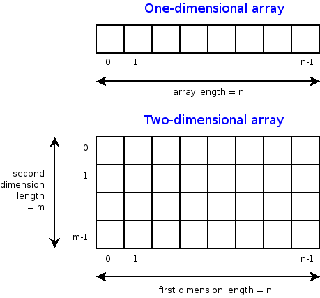
An array is a contiguous block of memory that stores multiple items of the same data type together. Here, each element will be efficiently located by its index, and the size is equal to the number of elements in the array, which must be fixed.

• We can easily calculate the position of each element by simply adding an offset (difference between the two indexes) to a base value (memory location of the first element of the array). So every element of an array can be accessed in O(1) time.
• We can easily calculate the amount of memory allocated to store an array because the size of the array is fixed, and all the elements are of the same type.

Most programming languages follow the standard of 0-based indexing, where the first element is present at the 0th index. On the other hand, sometimes we use 1-based array indexing, where the first element is present at index 1. For example, we use 1-based indexing in implementing array-based data structures like heap, segment tree, etc.

What are the different types of arrays?

One-dimensional array (1-D array)

In a one-dimensional array, elements are stored in a contiguous memory location, so the variable declared as an array is a pointer to the address of the first element of the array. This address is called the base address. 

We can calculate the address of any other element using this formula: Memory Address (A[i]) = Base Address (A) + Word Length * (i - First Index).

• Memory Address is the memory location of the ith array element.
• Base Address is the address of the first element of the array.
• Word Length is the number of bytes required to store one element depending on its data type, like character, integer, float, double, etc.
• First Index is the index of the first element of the array.

Two-dimensional array (2-D array)

A two-dimensional array is a tabular representation used to store elements in a rows and columns format. It is a collection of m x n elements, where m represents the number of rows and n represents the number of columns. To access any element in a 2-D array, two pieces of information are required: 1) The row index of the element and 2) The column index of the element.

We usually represent a 2-D array using a row-major representation, where array elements are stored row by row. All elements of the first row are stored in sequence, followed by the second row, then the third, fourth, and so on.

We can find the address of any element located at the ith row and the jth column using this formula: Memory Address (A[i][j])= Base Address(A)+ Word Length * (n * (i-1) + (j-1)).

Three-dimensional array (3-D array)

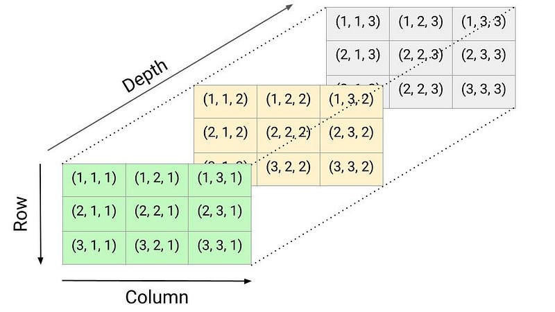
A three-dimensional array is an extension of a two-dimensional array with the addition of depth. We can visualize it as a cube with rows, columns, and depth as the third dimension. To access any element in a three-dimensional array, three pieces of information are required to identify the position of an element: 1) Depth index, 2) Row index, and 3) Column index.

We use 3D arrays in:

1. Computer graphics to represent the spatial coordinates of objects, vertices, and pixels of a 3D scene.
2. In medical imaging (MRI and CT scans) to store and process volumetric data. Each element in the array represents a voxel (3D pixel), which contains information about the properties of the corresponding point in the scanned object.
3. In scientific simulations to store and manipulate data from simulations like fluid dynamics, weather modelling, molecular dynamics, and simulations of physical systems.
4. In video games to represent the objects, terrain, characters, etc.
5. In data analysis and data mining to store multidimensional data sets.
6. In image processing applications like image segmentation, 3D reconstruction, etc.

Some popular array operations

Now we know the basic idea behind an array. Let's look at the various operations that can be performed on arrays:

• Traversal: Access elements in the array one by one.
• Insertion: Add an element at the given index.
• Deletion: Delete an element at the given index.
• Search: Search for an element in the array using the given index or value.
• Update: Update an element at the given index.
• Sorting: Arrange elements in increasing or decreasing order.
• Merging: Merge sorted arrays into a larger sorted array.
• Order Statistics: Find the kth smallest/largest element in an array.

Unsorted array: Search, Insert and Delete operations

Searching

In an unsorted array, we search elements using linear search.

//Pseudocode
int linearSearch(int A[], int n, int key)
{
    for (int i = 0; i < n; i = i + 1)
    {
        if (A[i] == key)
            return i
    }
    return -1
}

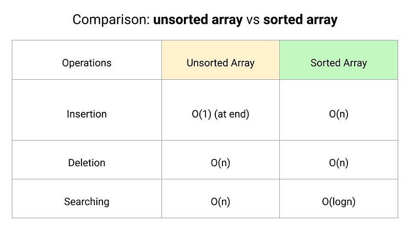
The worst-case time complexity of the linear search is O(n).

Insertion at the end

In an unsorted array, there is no order associated with the data elements. So we can directly insert elements at the end of the array. Suppose the size of the array is n and the index of the end element is endIndex.

• if(endIndex >= n), then the array is full and it is not possible to insert any element further. 
• if(endIndex < n), then there is some space left in the array and we can insert the element at endIndex + 1. As an output, we also return the new index of the end element which is endIndex + 1.

//Pseudocode
int insert(int A[], int endIndex, int key, int n)
{
    if (endIndex >= n)
    {
        print("Array is full. Element could not be inserted")
        return -1
    }    
    A[endIndex + 1] = key
    return endIndex + 1
}

The time complexity of the insert operation at the end is O(1).

Deletion

We first search for the element to be deleted using linear search. Let's assume that the linear search returns the index of the element in the array, which we store in the variable position.

• If position is equal to -1, then the element to be deleted is not present in the array.
• Otherwise, the element is present in the array. We delete the element by shifting all elements one position to the left, starting from the index position + 1 up to endIndex.

//Pseudocode
int delete(int A[], int endIndex, int key)
{
    int position = linearSearch(A, endIndex, key)
    if (position == - 1)
    {
        print("Element is not present in the array")
        return -1
    }
    
    for (int i = position; i < endIndex; i = i + 1)
        A[i] = A[i + 1]
    
    return endIndex - 1
}

Time complexity = Time complexity of the linear search + Time complexity of shifting elements to the left = O(n) + O(n) = O(n).

Sorted array: Search, Insert and Delete operations

Searching

In a sorted array, we search elements using the binary search.

//Pseudocode
int binarySearch(int A[], int l, int r, int key)
{
    if (l > l)
        return -1
    int mid = l + (r - l)/2
    if (key == A[mid])
        return mid
        
    if (key > A[mid])
        return binarySearch(A, mid + 1, r, key)
    else    
        return binarySearch(A, l, mid - 1, key)
}

The worst-case time complexity of the binary search is O(logn).

Insertion

In a sorted array, we first perform a search operation to find the correct position to insert the given element. For this, we can use linear search, which will take O(n) time in the worst case. But the array is sorted, so instead of linear search, we can use a modified binary search to find the position efficiently in O(logn) time.

Once we have identified the correct position, we insert the given element by shifting elements to one right.

//Pseudocode
int binarySearch(int A[], int low, int high, int element) 
{
    if (high <= low)
        return (element > A[low]) ? (low + 1) : low

    int mid = low + (high - low) / 2

    if (element == A[mid])
        return mid + 1

    if (element > A[mid])
        return binarySearch(A, mid + 1, high, element)

    return binarySearch(A, low, mid - 1, element)
}

int insertInSortedArray(int A[], int endIndex, int key, int n) 
{
    if (endIndex >= n) 
    {
        print("Array is full. Element could not be inserted.")
        return -1
    }

    int position = binarySearch(A, 0, endIndex, key)

    for (int i = endIndex; i >= position; i = i - 1)
        A[i + 1] = A[i]

    A[position] = key
    return endIndex + 1
}

Time complexity = Time complexity of the binary search + Time complexity of shifting elements to the right = O(logn) + O(n) = O(n).

Note: In an unsorted array, insertion is faster as compared to a sorted array because we don’t have to care about the position at which the element is to be placed.

Deletion

In the delete operation on a sorted array, we first search for the element to be deleted using binary search and then perform the delete operation by shifting the elements to the one left.

//Pseudocode
int deleteInSortedArray(int A[], int endIndex, int key) 
{
    int position = binarySearch(A, 0, endIndex, key)

    if (position == -1) 
    {
        print("Element is not present in the array.")
        return -1
    }

    for (int i = position; i < endIndex; i = i + 1)
        A[i] = A[i + 1]
        
    return endIndex - 1
}

Time complexity = Time complexity of the binary search + Time complexity of shifting elements to the left = O(logn) + O(n) = O(n).

Advantages of Array

Constant time random access: The index of each element in an array maps directly to a particular memory address. So we can access the element instantly if we know the index of the given element in an array.

Optimal use of memory: Arrays consist purely of data, so no space is wasted with links or other formatting information.

Sequential Access and Memory Locality: Most programming problems require iterating through all the elements of a data structure. So arrays are good for this because successive data elements are present in sequential order. This property helps us to implement high-speed cache memory on modern computer architectures.

Simplicity: Arrays are easy to understand, implement, and use in various applications.

Compatibility with Low-Level Languages: Arrays are a fundamental data structure supported by most programming languages, including low-level languages like C and C++. This makes arrays widely usable and accessible in various programming environments.

Disadvantages of Array

Along with their advantages, arrays also have some disadvantages:

Fixed Size: Arrays have a fixed size and the size of an array cannot be changed dynamically. In other words, we cannot adjust the size of the array in the middle of a program’s execution. For example, our code will fail soon as we try to add the (n + 1)th data element if we only allocate space for n data elements. 

Memory Wastage: Array requires allocating enough memory for the maximum number of elements upfront. This can lead to memory wastage if the allocated size is much larger than the number of elements actually stored. This inefficiency can be problematic in memory-constrained environments or when dealing with dynamic data where the size fluctuates over time.

Note: To solve the above problems, we can use the idea of the dynamic array where we can increase the array size dynamically as we need them.

Lack of Flexibility: Arrays have a fixed structure i.e. the elements must be of the same data type and size. This can be restrictive in scenarios where you need to store elements of different types or sizes.

Inefficient Insertion and Deletion: Inserting or deleting elements within an array (at the start or middle) can be inefficient. The idea is simple: We need to shift other elements, which will take O(n) time in the worst case. This inefficiency is problematic for large arrays or in the scenario of frequent modifications.

Sequential Structure: While the sequential access property of arrays can be advantageous, it can also be a limitation. If we need to search for a specific element that is not near the beginning or end of the array, we need to iterate through a significant portion of the array. This will result in slower search operations compared to other data structures like hash tables or binary search trees.

Array-based data structures

There are several array-based data structures that build upon the basic array concept to provide additional functionality and improved performance.

• Matrix: A two-dimensional array with rows and columns. It is used for representing grids, tables, or matrices.
• Dynamic Array: Also known as a resizable array, a dynamic array can dynamically resize itself to accommodate a variable number of elements. It combines the random access benefit of an array with additional advantages: Efficient memory usage with the ability to dynamically grow or shrink as needed.
• String: In many programming languages, strings are implemented as arrays of characters. It provides a convenient way to store and manipulate textual data with various string manipulation operations.
• Sparse Array: An array where most of the elements have the same default value, typically zero or null. To save memory, only non-default values are stored along with their indices. Sparse arrays are useful when dealing with large arrays where a majority of the elements are empty or have the same default value.
• Bit Array/Bitset: An array of bits where each element represents a single binary value, either 0 or 1. It is often used to represent a set of boolean flags or to optimize memory usage when dealing with large sets of boolean values.
• Array implementation of stack and queue: We can use array as an underlying data structure for implementing a stack or queue.
• Circular Buffer: An array-based data structure that wraps around the beginning when reaching the end. It efficiently supports both FIFO and LIFO operations and is often used in scenarios where a fixed-size buffer needs to be cyclically filled and emptied.
• Binary Heap: A binary tree-based data structure that is implemented using an array. It is used for efficient priority queue operations, such as extracting the min or max element.
• Hash Table: Hash tables use arrays as the underlying data structure. For example, the open addressing method of hashing use an array (bucket array) and hash functions to provide efficient key-value pair storage and retrieval.
• Binary Search Tree (BST) Array: Although binary search trees are implemented using linked structures, it is also possible to represent them using arrays. In this representation, each node is assigned an index, and the left and right child relationships can be calculated using mathematical formulas. Array-based BSTs have some advantages in terms of cache-friendliness and reduced memory overhead compared to linked structures.
• Segment Tree: A tree-based data structure used for efficient range queries and updates on a sequence of elements. It can be implemented using an array, where each node corresponds to a range of elements in the array.
• Fenwick Tree (Binary Indexed Tree): A tree-based data structure used for efficient range queries and updates on an array. It can be represented using an array where each element corresponds to a specific range of elements in the original array.
• Adjacency Matrix Representation of Graph: In the adjacency matrix representation, a two-dimensional array is used to store the edges between vertices. If there is an edge between vertices u and v, the corresponding cell in the matrix is marked as 1 or contains the weight of the edge. If there is no edge, the cell is marked as 0 or can contain a special value to indicate absence.

Popular array-based problem-solving approaches

• Building partial solutions using a single loop
• Two-pointers approach
• Sliding window approach
• Divide and conquer approach
• Decrease and conquer
• Using binary search
• Direct addressing and hashing
• Using sorting and loop
• Using prefix array and loop
• Bit manipulation approach

Application of array

• Arranging a particular type of data in a sequential arrangement: storing contacts on our phone, storing speech signals in speech processing, etc.
• Implementing various data structures like stack, queue, adjacency matrix representation of graphs, hash tables, binary heaps, etc.
• Many sorting and searching algorithms like binary search, exponential search, quicksort, and merge sort, rely on arrays for efficient data manipulation.
• We use arrays in cryptographic algorithms for storing and manipulating encryption keys, cypher texts, and other data structures involved in secure communication and data protection.
• Arrays are fundamental to numerical computations and scientific computing. They provide a structured way to represent vectors, matrices, and tensors used in mathematical calculations, simulations, and data analysis.

Critical ideas to think!

• Which Indexing is more efficient: 0-based indexing or 1-based indexing?
• How does a dynamic array solve fixed array size problems?
• What type of data structure do we use to store multiple types of items in a continuous memory location?
• How can we find the length of an array, given only the name of the array?
• How can we insert or delete a new element at the beginning of an unsorted or sorted array?

Suggested array-based problems to practice

• Move zeroes to end of an array
• Find the minimum and maximum value in an array
• Sort an array in a waveform
• Valid Mountain Array
• Sort an array of 0s, 1s, and 2s
• Container With Most Water
• Remove duplicates from sorted array

If you have any queries or feedback, please write us at contact@enjoyalgorithms.com. Enjoy learning, Enjoy algorithms!