Naive Bayes Classifier: Supervised Machine Learning Algorithm

In Machine Learning and Data Science field, researchers have developed many advanced algorithms like Support Vector Machines, Logistic Regression, Gradient Boosting, etc. These algorithms are capable enough to produce very high accuracy. But among these advanced ones, there exists an elementary and Naive algorithm, known as Naive Bayes. 

In English, the "Naive" word is used for a person or action lacking experience, wisdom, or judgment. This tag is associated with the Naive Bayes algorithm because it also makes some silly assumptions while making any predictions. But the most exciting thing is it still performs better or equivalent to the best algorithms. So let's learn about this algorithm in greater detail.

Key takeaways from this blog

• What is Bayes theorem?
• Why Bayes theorem in Machine Learning?
• Naive Bayes examples for single and multiple features.
• How does Naive Bayes handle the non-categorical features?
• What is Gaussian Naive Bayes?
• Python-based implementation
• Advantages and disadvantages of Naive Bayes.
• Industrial applications of Naive Bayes.
• Possible Interview Questions on this topic.

Let's start without any further delay.

Note: In our probability blog, we discussed Baye's theorem.

Why Bayes Theorem in Machine Learning?

Let's try to find the answer to this question. In the case of supervised learning, we have input features and the corresponding output labels present with us. We try to make our machines learn the relationship between input features to the output variable. Once this learning is done on training data, we can use this model to make predictions on test data. Let's represent this supervised approach in a Bayesian format. 

We know the feature values for test data and want to see the output label if that particular values of features are present. We can also say we want to predict the chances of occurrence of any label if the values of features are already known. That is precisely the same as p(label | feature). From the Bayes theorem, to know the value of p(label | feature), we must know the likelihood probabilities p(feature | label) and the prior probabilities, p(label) and p(features). But, do we really have these values?

Yes! from the training data. That's the whole crux of supervised learning. Right?

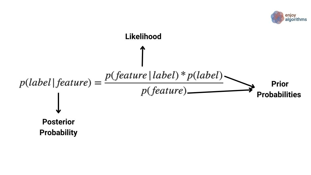
Let's discuss the terms on the right side of the formulae above. The likelihood term p(feature | label) says the probability of that feature if we already know the label. And for training data, we know the label for each sample. Also, the prior probabilities p(label) and p(feature) can be calculated from the training data. So ultimately, we will have the posterior probability that we wanted to calculate.

Naive Bayes example

Single Feature

Let's take the example of a football game, and below is the data which says if humidity is high or normal, then play happens; otherwise, if humidity is low, the play does not occur. Straightforward data, correct?

Suppose we want to make a machine learning model, which receives the feature value of humidity and tries to predict whether the play will happen or not. So suppose we know the humidity as Normal, and let's calculate the chances of play happening, i.e., p(play = Yes | humidity = Normal).

From the data:

p(humidity = Normal | play = Yes) = Probability of humidity to be normal when we know that play happened is 1/2, as there are two cases when the play happened. One is when humidity = High and Humidity = Normal. So the probability of humidity = Normal will be 0.5.

p(play = Yes) = Probability of game to have happened will be 2/3 as we have 3 samples out of which 2 say the play happened as "Yes".

p(humidity = Normal) = probability of humidity to be normal will be 1/3 as there are three samples out of which 1 instance is of humidity = Normal.

The same can be understood from the data intuition as well. Similarly, p(play= No | humidity = Normal) can be calculated, and it will be 0.

Multiple Feature

The example we saw above had just one feature, the humidity value. But in the practical, real-life data, we will have multiple features. In such a case, the same equation can be represented as,

Expanding the above equation,

This calculation is extensive and expansive in terms of computations. That's where the Naïve Bayes algorithms come with their "naive" assumption. It considers every feature is independent of each other, which means one feature is unaffected by the occurrence of any other feature. 

This assumption is impractical in real-life scenarios. Suppose we are recording features from our cell phone's battery, the terminal voltage, current, and temperature. Using these, we estimate whether battery health is "good" or "bad". It's a classification problem statement, and algorithms like SVM, logistic regression, etc., will learn mapping functions between feature sets and labels. While learning, these algorithms will not assume that current is independent of the Voltage feature, which is oblivious. Voltage produces the current, which results in the heating of the battery, so temperature varies accordingly. So all features are dependent. 

But Naive Bayes algorithm assumes that all three features are independent, and the occurrence of one feature is totally unaffected by the occurrence of others. This is not true in practical cases. Still, this algorithm produces quite fascinating results. According to Naïve Bayes, the above equation is modified as follows:

This assumption drastically reduces the computation cost and also delivers good accuracy. Also, in the Naive Bayes algorithm, we don't calculate the denominator of the above equation to save some computation power. Because, for all the classes, the denominator term remains the same and does not make any contribution in segregating different classes. Hence, we can represent the above equation as:

How does Naive Bayes handle the non-categorical features?

What if the features are continuous numerical values (non-categorical). How will we estimate probabilities in such a case? 

Here comes the theory of Probability Distribution Function (PDF). We need to estimate the probabilities for numerical variables using this concept.

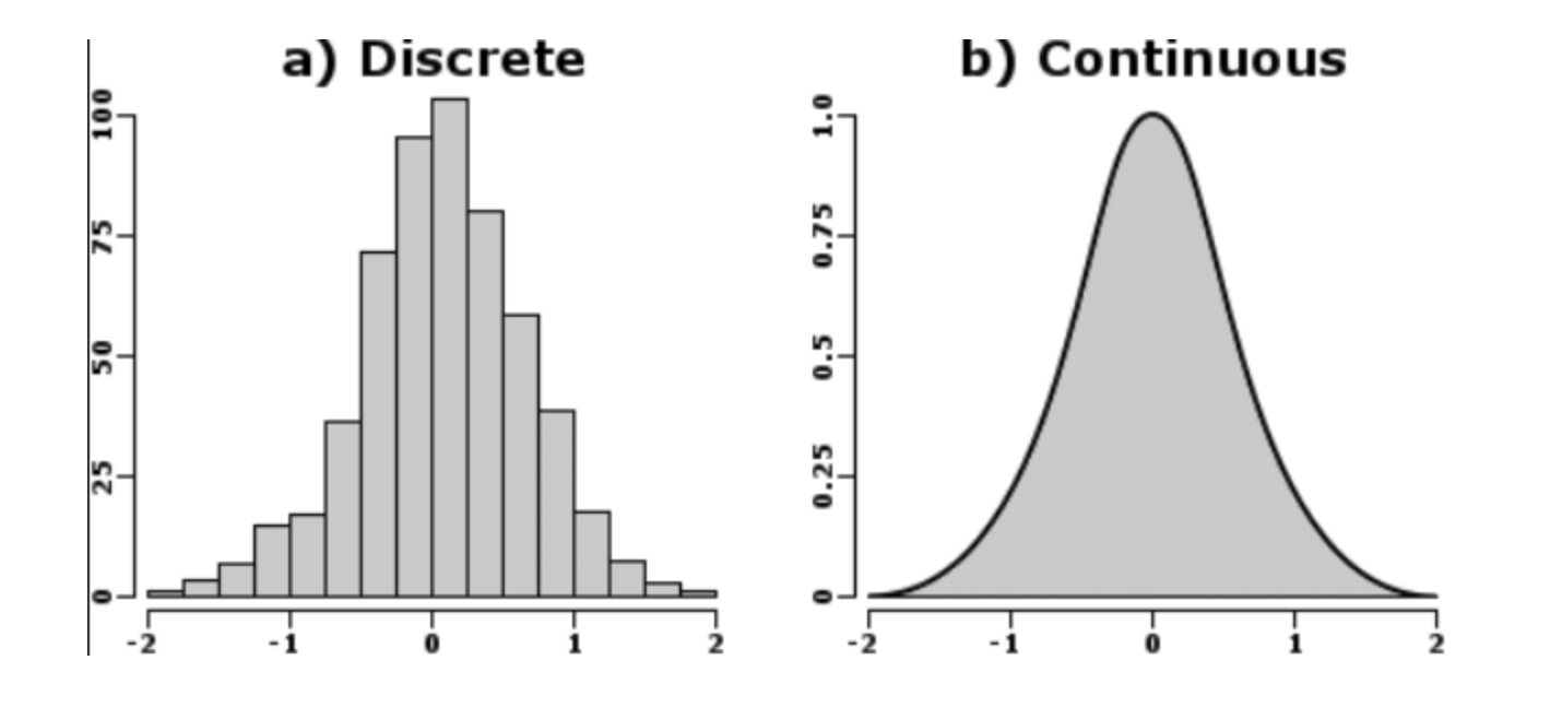
Suppose we assume that the PDF is a gaussian or normal distribution. In that case, we need to calculate the mean(μ) and standard deviation (σ) of that feature,and then for any value of feature x, the probability f(x) can be calculated from the below equation.

Gaussian Naïve Bayes

In the case of gaussian distribution assumption, we call Naïve Bayes, Gaussian Naïve Bayes algorithm. We can choose other probability distribution functions, like Bernoulli, Binomial, etc., to estimate probabilities. Among all these, gaussian is the most famous one as most of the real-world sensors produce data in the gaussian distribution format. If we look at the image below closely, most people in the gym use 15–20 Kg weights. Later on, the usage of other weights decreases subsequently, like what we observe in the gaussian distribution.

Too much theory, let's implement it on a practical machine learning application, i.e., Sentiment analysis.

Can we solve regression problems using Naive Bayes?

Although the native form of the Naive Bayes algorithm is made to solve the classification problems only, a team tried to solve the regression problem using Naive Bayes, and the work can be found here. They concluded that they did not achieve good results and suggested that Naive Bayes is suitable for classification algorithms.

Naive Bayes Sklearn In Python

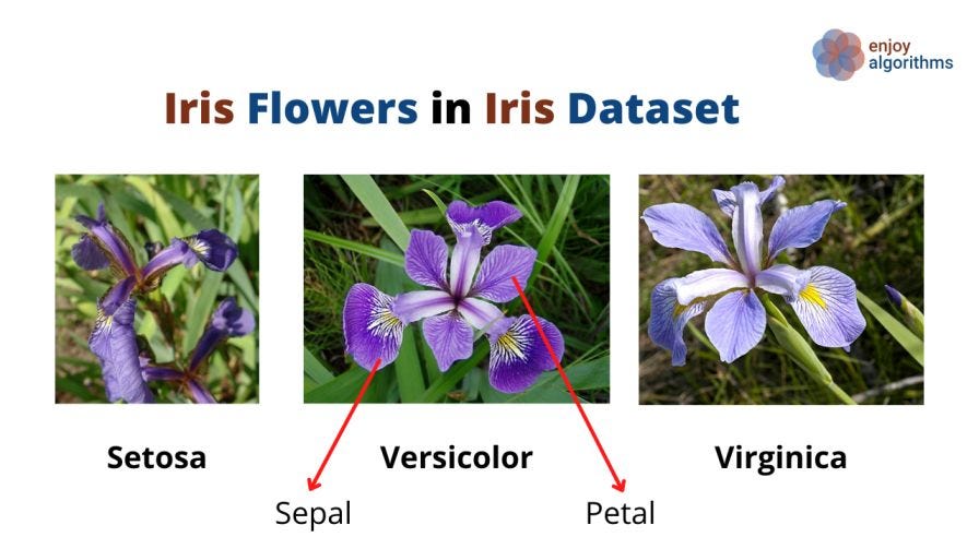
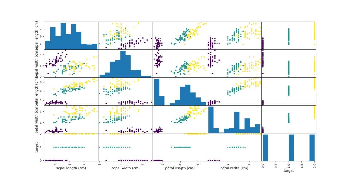
Let's train a Naive Bayes algorithm on the famous Iris dataset. The objective of our algorithm would be to look at the available features like Sepal/Petal length/width and classify flowers into three categories of Setosa, Versicolor, and Virginica.

Step 1: Importing required libraries

Standard libraries like numpy (for numeric operations), pandas (for managing the data), and matplotlib (to visualize the analysis of the dataset) would be required.

import numpy as np
import pandas as pd
import matplotlib.pyplot as plt

Step 2: Loading the dataset and visualizing scatter-plot of features

The famous iris dataset comes with the Scikit-learn library. If we print the features present in the dataset, the output is ['sepal length (cm)', 'sepal width (cm)', 'petal length (cm)', 'petal width (cm)']. Also, the target variable y can take three values [0, 1, 2] corresponding to three flower classes.

from sklearn import datasets

iris = datasets.load_iris()            #loading dataset

X = iris.data[:,]                    #input
y = iris.target                      #target

print("Features : ", iris['feature_names'])

iris_dataframe = pd.DataFrame(data=np.c_[iris['data'],iris['target']],
                             columns=iris['feature_names']+['target'])

plt.figure()
grr = pd.plotting.scatter_matrix(iris_dataframe, c=iris['target'],
                                  figsize=(15,5),
                                  s=60,alpha=8)
plt.show()

# Features :  ['sepal length (cm)', 'sepal width (cm)', 'petal      # length (cm)', 'petal width (cm)']

The code above will plot the diagram shown below.

Step 3: Visualizing the correlation and checking the assumption of Naive Bayes

We can plot the correlation matrix using the seaborn library.

import seaborn as sns
dataplot = sns.heatmap(iris_dataframe.corr(), annot=True)

plt.show()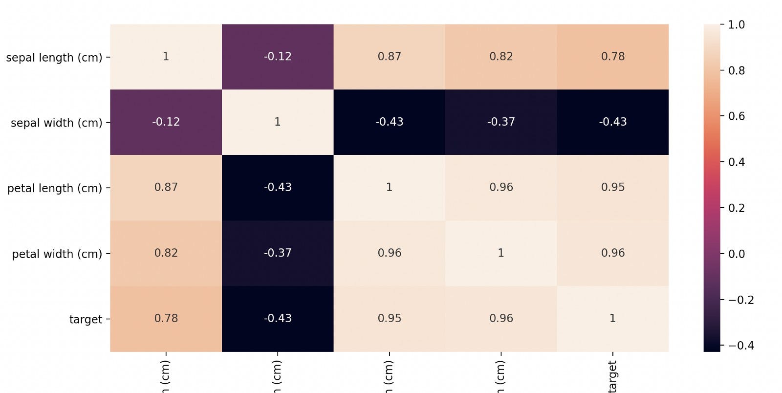

We can see that the features are highly correlated. But as per Naive Bayes assumption, it will treat features as entirely independent of each other. Based on this, our algorithm will compute the following probability for all three flower classes.

Step 4: Split the dataset

Now we are in a position where we can segregate our training and testing data. For that, we can use the inbuilt function of traintestsplit from Sklearn.

from sklearn.model_selection import train_test_split

X_train, X_test, y_train, y_test = train_test_split(X,y,test_size=0.25,random_state=0)

Step 5: Fit the model

Now, assume our data follows Gaussian distribution and import the Gaussian Naive Bayes GaussianNB model from Sklearn. Let's fit this model into our training data.

from sklearn.naive_bayes import GaussianNB

NB = GaussianNB()
NB.fit(X_train, y_train)

Hurrah! We have our model ready with us now.

Step 6: Evaluate the model

We must know that we have solved a classification problem to evaluate the model. Hence some standard metrics for evaluating our model can be accuracy, precision, recall, F-1 Score, etc. A detailed list can be found here in this blog. As we know, all these matrices can be calculated by having the confusion matrix ready with us. So let's plot the confusion matrix.

Y_pred = NB.predict(X_test)

from sklearn.metrics import confusion_matrix
cm = confusion_matrix(y_test, Y_pred)

df_cm = pd.DataFrame(cm, columns=np.unique(y_test), index = np.unique(y_test))

df_cm.index.name = 'Actual'
df_cm.columns.name = 'Predicted'

sns.heatmap(df_cm, annot=True)# font size
plt.show()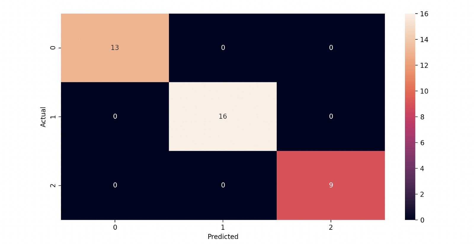

From the matrix, we can see that the model quickly achieved 100% accuracy on test data. This is really amazing. It started with the silly assumption but provided whatever we wanted. That's the main reason why this algorithm is famous among researchers.

Advantages of Naive Bayes

• Computationally Simple: This classifier is computationally very simple compared to algorithms like SVM and XGBoost. 
• When the independent nature of features becomes true in data, the Naive Bayes algorithm performs the best and can beat the accuracy of Logistic Regression.
• Multi-class prediction: It can provide us with the probabilities do different classes and hence can give multi-class predictions.
• It works best in the case of Categorical variables compared to the numerical ones.

Disadvantages of Naive Bayes

• Independent treatment of features: One of the most significant disadvantages of this algorithm is that it treats every feature independently, which can be cumbersome most of the time. Advanced classifiers like SVMs learn the relationship between the feature and target variables and the relationship among features. This is not the case with Naive Bayes.
• Zero frequency case: Probably, some values from a categorical variable do not appear in training data. In such a case, Naive Bayes will assign a zero probability to these samples when they appear in test data. This is called "Zero Frequency" and can be cured using smoothing techniques, like Laplace estimation.
• Bad Estimator: Naive Bayes is considered to be a lousy probability estimator, so we should not take the probability predicted by this algorithm too seriously. 

Industrial Applications of Naive Bayes

This algorithm is naive, but because of its performance, several industrial applications are based on this.

• Recommendation System: Collaborative Filtering and the Naive Bayes algorithm form the recommendation system that can recommend some products/movies/songs to users.
• Multi-class prediction: One of the most significant advantages of Naive Bayes is its applicability in predicting the probability of multiple classes. 
• Real-time prediction: Because of its lesser complex nature, it can give prediction results very fast. Many advanced algorithms like SVM XGBoost are too heavy sometimes for smaller classification tasks. In such a scenario, Naive Bayes performs well.

Possible Interview Question

The theory of this algorithm is really important as it is rare to find full-scale projects in resumes related to this algorithm. Interviewers want to test the probability knowledge of this topic. Some popular questions can be:

• Explain the Bayes Theorem and associate it with the Naive Bayes algorithm.
• Why is this algorithm called Naive?
• How do these probability calculations hold for continuous numerical variables?
• What is Gaussian Naive Bayes algorithm? What variants can be possible or why Gaussian?

Conclusion

In this article, we learned about the Naive Bayes classifier in detail. We drew the intuition from Baye's theorem of probability and stated its correlation with the Naive Bayes algorithm. We also saw the python implementation of this algorithm using sklearn. In the last, we discussed the advantages, disadvantages, and industrial applications. We hope you enjoyed the article.

Enjoy learning, Enjoy algorithms!