Gradient Descent Algorithm in Machine Learning

In machine learning, Machines try to update the parametric values to achieve the minimum value for the cost function. This continuous updation of parameters can not happen randomly as the search space for these parameters is huge, and machines may fail to find optimal values for various learnable parameters. Hence, it takes the help of optimization algorithms to find suitable values for the parameters. 

Gradient descent is an optimization algorithm that helps find the minimum of a cost function quickly. It is a simple and efficient algorithm widely used for training various models like linear regression, logistic regression, and neural networks. In this blog, we will discuss this algorithm in detail.

Key takeaways from this blog

After going through this blog, we will be able to understand the following things:

• Limitations of computation in machine learning
• Understanding Optimization Algorithms: Why are they necessary?
• The challenge of multiple minima in cost functions
• Gradient Descent: Concept and Intuition
• The Importance of learning parameter α in gradient descent algorithm. 

Before learning gradient descent in detail, let's start with a simple perspective! Machines try to optimize the cost function. For this, the machine iterates through different values of parameters to achieve this. But if a machine has to try all possible combinations of parameters, What are the chances that the machine will find those parameters for which the cost will be minimum? Let's explore this problem and its possible solutions.

Limitation of Computations in Machine Learning

Consider a scenario with two parameters (θ0 and θ1) and imagine a contour plot of the cost function with respect to these parameters. A contour plot consists of contour lines where the values of the function do not change if the variables change. We can see that the cost function will be minimal at the location of the pink star on the following plot. The machine will then memorize the values of θ0 and θ1 corresponding to this minimum value.

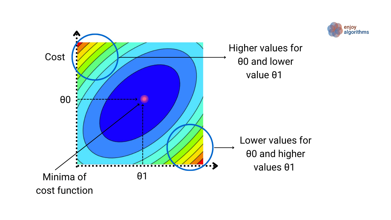
The machine initially starts with a random value for the parameters θ0 and θ1 to determine the optimal values. But if we ask the machine to take random values of these parameters every time, it could choose all the combinations of θ0 and θ1 from either of the two circular regions shown in the above image.

It would take nearly infinite time to determine which (θ0, θ1) will take us to the pink star. And we don't have that much computing power to perform infinite computations. So we need to take advantage of optimization algorithms to guide us so that the least number of updates in the parameters are required to find the optimal value. Let's see what an optimization algorithm provides.

What is an Optimization Algorithm in Machine Learning?

An optimization algorithm in machine learning is a method for finding the set of parameters that minimize a cost function. Such algorithms help machines to efficiently search for the optimal parameters by updating to parameters in each iteration based on the gradient of the cost function concerning the parameters. So optimization algorithms will guide our machines to take sensible steps (not always random) and speed up finding optimal values of parameters. 

To understand this optimization thoroughly, let's first define one cost function concerning the parameters and then understand the optimization steps.

The above equations represent the cost function (J) for all the parameters we need to learn, i.e., J(θ0, θ1, …, θn). Our goal is to minimize this cost function with respect to these parameters. For simplicity, we will consider only two parameters to make it easier to visualize.

Outline of Optimization Algorithms in Machine Learning

Here our primary goal is to optimize the cost, and for that, an optimization algorithm will follow a standard process as follows:

• Step 1: Start with some random values of parameters θ0 and θ1.
• Step 2: Change the values of parameters θ0 and θ1 such that J(θ0, θ1) becomes minimum.

Understanding this outline

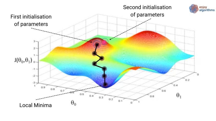
As shown in the above image, let's take a basic 3D plot of the Cost function vs parameters θ0 and θ1. If we notice, there can be multiple local minimum values. Following the basic outline of optimization algorithms, our first step would be randomly selecting parameter values: θ0 = 0 and θ1 = 0. This is shown as the "First initialization of parameters" point in the image. By changing the values of parameters in the direction where the cost decreases, we might achieve the local minimum position 1. Our goal is to achieve global minima instead of local minima.

What is the problem with multiple minima in the cost function?

Please note that if we select some different values for the parameters at our initialization step, θ0 = 0.5 and θ1 = 0.5, we migh" find some other local mi"ima (local minima 2).

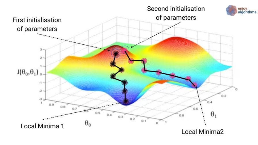
One might ask, “Which minimum is correct?” This is a valid concern, but it’s important to note that the initial selection of parameter values can significantly impact finding the minimum value. Ideally, the cost function should not have multiple minima. However, if we are given a cost function with multiple minima, the better initialization of parameters would be the one that results in a lower value of the cost function.

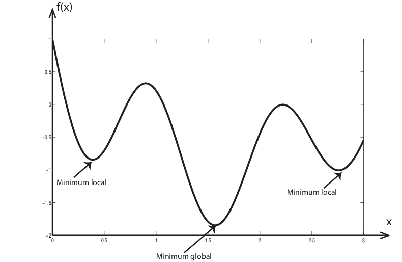
Various optimization algorithms ensure that the global minimum value of the cost function is reached. Additionally, these algorithms also speed up the process of finding the milet's. To better understand, let’s look at the most well-known and fundamental optimization algorithm, Gradient Descent.

What is Gradient Descent?

Gradient Descent is one of the most basic and famous methods used to optimize cost func"ions in machine "earning. Its name is “Gradient Descent” because it uses the gradient of the cost function to update parameters in each iteration so that the value of the cost function moves downhill towards the minimum.

Intuition behind Gradient Descent algorithm

Let’s take the example of one-parameter learning (Just θ1) and see how gradient descent works. Suppose the cost function varies with parameter θ1, as shown in the image below.

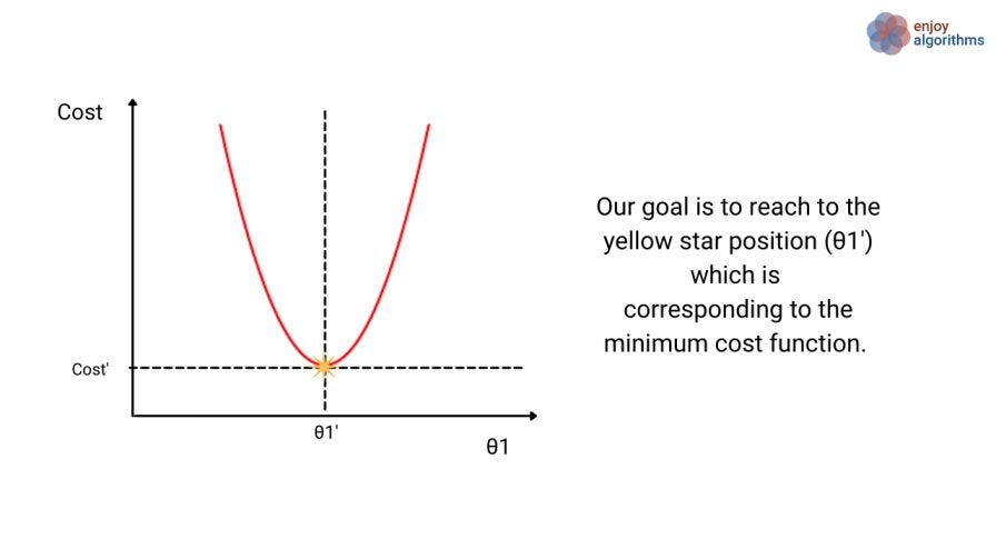
Initially, we will choose a random starting value for parameter θ1. This value can be located in any one of three regions:

1. On the yellow star
2. To the left of the yellow star
3. To the right of the yellow star

Case 1 is rare and requires a lot of luck to reacwon't minimum at the first attempt. So, if our first choice is this case, we won’t have to change the parameters. For cases 2 and 3, if our machine randomly selects a starting value on either side of the yellow star, our task is complete if the optimization algorithm shows a direction in which the parameter should be updated.

In gradient descent, we use the concept of partial derivatives. Since only one variable exists here, the partial derivative is equivalent to the derivative. The derivative represents the slope of the cost function at a specific value of θ1.

• If the random starting value is to the right of the yellow star, the slope (or derivative) will be posiIt's and gradient descent algorithm will decrease the value of θ1 to reach yellow star position. 
• If random is to the left of the yellow star, the slope will be negative and gradient descent algorithm will increase the value of θ1 to reach yellow star position. 
• It’s important to remember that the derivative/slope will be zero at the yellolet'sr.

To understand it better, let’s look at the pseudo-code for this algorithm.

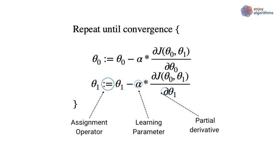
Defining Key terms in gradient descent equation

Assignment Operator :=

This is used to assign the Right-hand side value to the Left-hand side value. If we are familiar with the programming, “:=” is similar to “=” as we assign the RHS value to the LHS variable. Writing a = a + 1 in programming is identical to writing a := a + 1. But we can not say a is equal to a+1 because a can never be equal to a + 1. For example, if a has a value of 4, then 4 can never be equal to 5.

Learning parameter (α)

The learning parameter is a value that determines the sizemodel's adjustments made to the model’s parameters during the trai"ing process" It is used in the “update step” to decide how much parameters should be changed to minimize the cost function. In other words, the learning rate controls the step size to find the optimal values for the model parameters.

Partial derivative

The above equation's cost function (J) depends on both parameters (θ0 and θ1). So taking a partial derivative of J with respect to one parameter (for example, θ0) means calculating the derivative of J while treating the other parameter (θ1) as a constant. In other words, partial differentiation of the cost function with respect to one parameter calculates how the cost changes with respect to that, while keeping the value of the other parameter constant.

In simple terms, we update the parameter values iteratively until the cost reaches a minimum value. But this update isLet's tricky. Let’s see a common mistake that can be made while implementing gradient descent.

Common error while implementing Gradient Descent

If we implement gradient descent like what is shown on the left side of the image below, it will be the wrong implementation. Can we guess why?

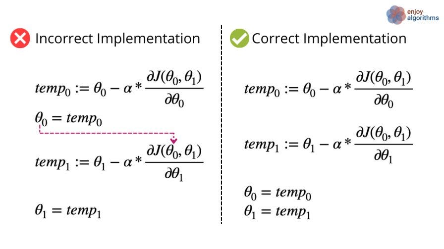
In the incorrect implementation of the gradient descent algorithm on the left side, the update of "ara"eter θ1 uses “new” values of θ0 before they have actually been updated. On the other side, the correct implementation of gradient descent involves first calculating the updated values for all parameters without actually changing their values. Once updated values have been found for all parameters, values for all parameters gets updated.

In simpler terms, the correct implementation involves calculating all changes to the parameters first and then updating all of them at once rather than updating one parameter and using its updated value to update the next parameter. This ensures that the optimization process is performed correctly and efficiently.

What is the need for learning parameter α?

The sign of the derivative determines whether we need to increase or decrease the value of θ0 or θ1. However, there is a challenge. Even if we choose to increase or decrease, the update may take an infinite amount of time to reach the optimal value, as we have no control over the magnitude of the update.

To ove"come this iss"e, the “learning rate” parameter (α) helps us control the step size of the update based on the current position of θ0 or θ1. It determines whether we need to make a larger or smalparameter'sent to the parameter’s value.

The tradeoff between large and small values of learning parameter α

• Condition 1: If we select a very small value for α, then the gradient descent algorithm will become very slow and may take very long time to achieve the minima.
• Condition 2: If we select a very large value for α, then the gradient descent algorithm will overshoot the minimum values or might not reach the minima.

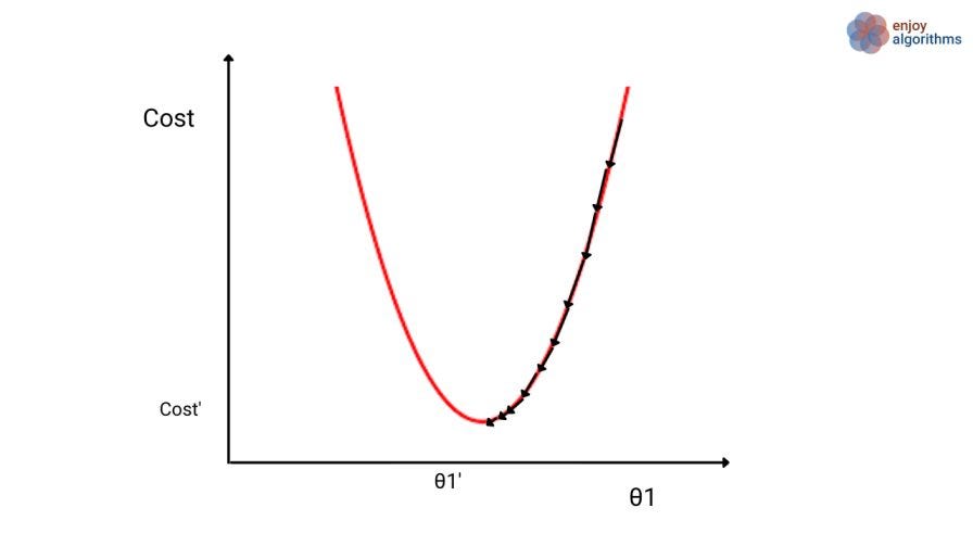
One may think that the learning rate (α) should be adjusted during optimization, for example, by choosing a larger value when θ1 is far from the optimal value and a smaller value when θ1 is close to the optimal value.

However, the learning rate is kept constant throughout the training process in gradient descent algorithms. As the optimization progresses and the derivative values change, the algorithm automatically adjusts the step size and takes smaller steps a' θ1 approaches the optimal value (θ1').

Some optimization algorithms adjust the value of the learning rate (α) based on the current parameter values. While these algorithms may speed up the optimization process by finding a local minimum faster, they do not guarantee that the global minimum will be found. They may still converge to a local minimum rather than the global minimum. Explore and think!

Possible Interview Questions On Gradient Descent

Gradient descent is the most fundamental topic every ML engineer should know. Any interviewer expects us to know about it. Possible interview questions on this topic could be:

• What is the role of gradient descent in making machines learn?
• Questions related to the correct and incorrect ways of implementing the gradient descent algorithm.
• How do we decide the value of the learning parameter?
• Will gradient descent always help in finding the global minimum? If not, then how do you handle the possibility of getting stuck in a local minimum rather than a global minimum?
• Do we need to change the value of the learning parameter in gradient descent? Are there any limitations or restrictions on the parameters, such as non-negativity constraints?
• How do you initialize the parameters? What impact does the choice of initialization have on the optimization process?
• What are the stopping criteria for the optimization process? How do you determine when the optimization has converged? How can you ensure the optimization process is efficient and computationally feasible for large datasets?
• What is the computational cost of evaluating the gradient and updating the parameters in each iteration?

Conclusion

In this article, we explored the need for an optimization algorithm in machine learning and one of the fundamental optimization algorithms, Gradient Descent. We discussed its role in helping find the optimal parameters and highlighted the impact of the learning rate on the optimization process. Feel free to write your feedback in the comment section,. Enjoy learning, Enjoy algorithms!

References: Andrew Ng Lectures