Principal Component Analysis (PCA) in Machine Learning

Introduction

Data lies in the heart of Machine Learning and Data Science. During data collection, we generally record multiple attributes for the sake of not-loosing any critical information. For example, if there is a requirement of collecting weather data, we record various attributes like humidity values, atmospheric pressure, temperature, wind speed, etc. It may be possible that we will not use all of them for the model building process. Still, we collect all of them because if a project has some special requirements and we don't have that attribute, we will have to start the collection process from scratch. 

We record multiple features, but at the same time, we have limitations with the compute capabilities. Using all the recorded features to build our machine learning models is never a good practice. It will make machine learning models too heavy and might become impractical to use for real-time applications. Also, the analysis of data having multiple features is a cumbersome task. That's where the technique of dimensionality reduction comes into the picture. In this article, we will discuss one such method of dimensionality reduction, Principal Component Analysis, popularly known as PCA.

Key takeaways from the blog

• Why do we need dimensionality reduction techniques?
• What is Principle Component Analysis?
• What are the steps to implement the PCA algorithm?
• Why do we need to standardize data before PCA?
• What is the Scree plot in PCA?
• Comparison with Scikit-learn implementation.
• What are the assumptions we make in PCA?
• Where do we use PCA?
• Possible interview questions on this topic.

Let's start without any further delay. 

Why do we need dimensionality reduction techniques?

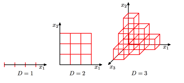
The first thought that would come to our mind is "Plot the graph of one attribute with respect to the other attribute". Via this way, we will be able to identify the underlying relationships. That's correct. But what if we say that there are ten attributes in data, and we need to analyze their relationships. Will the answer still be the same? 

We can say, Yes! The answer would remain the same. We can use 2D plots for every two pairs, i.e., selecting two attributes among 10. From combination theory, the same can be written as:

Really? Will it be easy to analyze 45 different plots and then find the overall relationships among all of them? No! Right? That's where dimensionality reduction algorithms come into the picture, where we bring the higher dimensional data into lower dimensions without losing "much" information. The meaning of this "much" term will be evident in a while. PCA (Principal Component Analysis) is one such technique for dimension reduction.

What is Principle Component Analysis?

Let's first define it formally: Principal Component Analysis (PCA) is an unsupervised machine learning technique to reduce the dimensionality of data consisting of a large number of inter-related attributes (or features or variables) but at the same time retaining as much as possible of the variation present in the original data.

Every attribute in the data is considered as a separate dimension. The PCA algorithm transforms the data attributes into a newer set of attributes (or features or variables) called Principal Components (PCs). Considering the same example above, if we have ten attributes in the data, the PCA algorithm will form a new set of 10 attributes using the earlier ten attributes. This new set of attributes will be called PCs. But we might think that if we still have ten attributes, how did we reduce the dimension?

That's the exciting part of PCA. With the earlier set of attributes, we were not sure about the relationships, but with the new set of PCs, we know two significant properties among them:

• These PCs are "uncorrelated," or we can say, the dimension corresponding to one PC is perpendicular to the dimension corresponding to all other PCs. So if we calculate the dot product between two PCs, it will be zero.
• These PCs are arranged (ordered/placed) such that the first few PCs from the start retain most of the variations present in the original set of attributes.

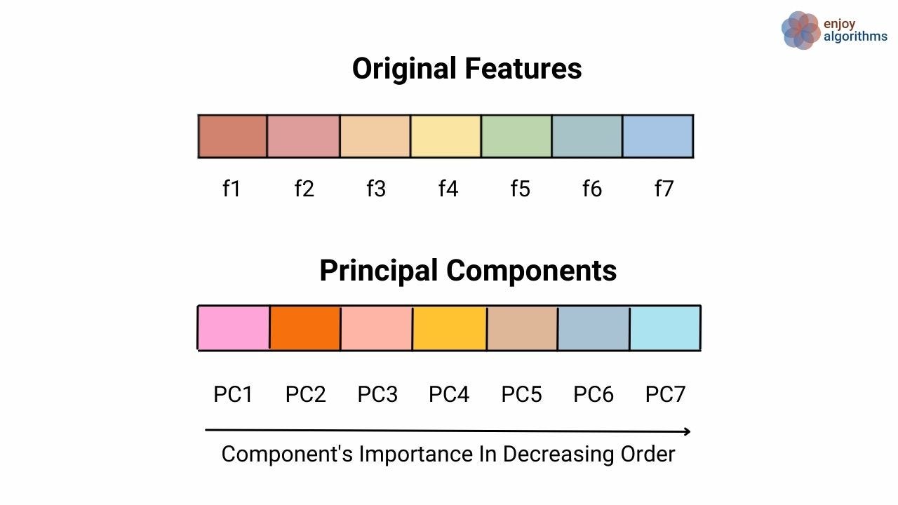
If we want to reduce the dimensionality, we can remove some PCs from the last. Some information will get lost, but this loss will be insignificant as most of the variation is retained by PCs present at the start. That's why we used the term "much" earlier. Also, note that we correlate the term "variation" with the term "information" as attributes having maximum variations contain more information than others. So, in the last, if we need to summarize, we can say that PCA is an unsupervised, non-parametric, and statistical machine learning approach used to reduce dimensionality.

The term PCA was first coined by Pearson in 1901 and later developed independently by Hotelling in 1933. Although it originated from multivariate data problems, now it has a broader range of applications like denoising signals, blind source separation, and data compression.

What are the steps to implement the PCA algorithm?

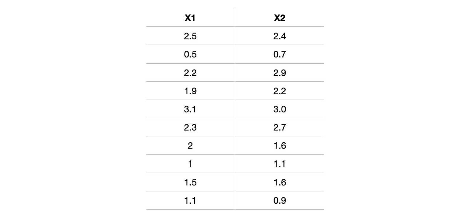
The best way to understand the whole outflow is to implement it step-wise. Let's quickly pick one data and try to implement it. For better visualization of reduction, let's first choose a dataset having only two attributes, X1 and X2. Selecting a simple case would be better as we realize or feel the dimension reduction.

#Import Libraries
import numpy as np
from matplotlib import pyplot as plt

#Defining attributes
x1 = [2.5,0.5,2.2,1.9,3.1,2.3,2,1,1.5,1.1]
x2 = [2.4,0.7,2.9,2.2,3.0,2.7,1.6,1.1,1.6,0.9]

#Plotting Attributes in 2 D plane
plt.figure("X1 vs X2")
plt.plot(x1,x2,'*')
plt.xlabel('X1')
plt.ylabel('X2')
plt.show()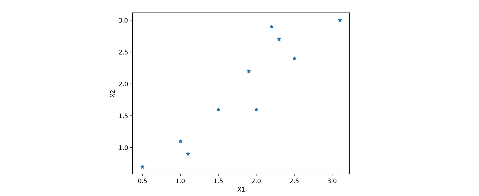

This article will be using Eigenvalues and Eigenvectors to find the principal components for our data and reduce dimensionality. If you are not familiar with these terms, we recommend looking at this Linear Algebra article. Now let's move towards the PCA steps.

Step1: Standardization Of Data

Calculate the deviation of every element from the mean of corresponding attributes. i.e., X1-mean(X1) and X2-mean(X2) and then divide the result by the standard deviation of that attribute. This standardization is also known as Z-Mean.

#Calculating Z-mean of attributes and forming the standardized data
Z1 = (x1-np.mean(x1))/np.std(x1)
Z2 = (x2-np.mean(x2))/np.std(x2)
Z3 = np.array([Z1.T, Z2.T])

'''
Standard Deviation of X1 = 0.7449161026585478

Standardized X1 = [ 0.92627881, -1.7585873, 0.52354889, 0.12081898, 1.73173864, 0.6577922, 0.25506228, -1.08737078, -0.41615425, -0.95312747]

Standard Deviation of X2 = 0.8030566605165541

Standardized X2 = [ 0.61016865, -1.506743, 1.23278973, 0.36112022, 1.35731394, 0.9837413, -0.38602507, -1.00864614, -0.38602507, -1.25769457]
'''

Why standardize the data in PCA? Why mean centering?

Mean-centering (subtraction from the mean) of the input data before estimating eigenvalues and eigenvectors is integral to the algorithm. This was one of the most debatable topics since the discovery of PCA. In 2003, researchers justified that the mean centering ensures that the first principal component is proportional to the maximum variance of the input data. 

Suppose we want to revert to the original set of attributes, but we already have removed some PCs. So there will be some loss in the original data as well. We will not be getting the "exact" same attributes, but we can approximate the values using the basis function. Mean centering is justified in finding a basis function that minimizes the mean square error approximating the original data.

Why division with standard deviation?

Division with the standard deviation of the original feature ensures that the standard deviation of standardized data becomes 1. This will make the importance of all the attributes equal, and our algorithm will not be biased towards any specific feature. We must not forget that the overall goal of PCA is to transform the data such that it retains most of the information/variance. 

To understand it, let's suppose the variance of X1 would be 1, and the variance of X2 would be 20. In such a scenario, 20 is very high with respect to 1, and hence, our principal component will overlap (or be biased towards) X2 and ignore X1 because X2 contains most of the variance. Therefore, to give importance to all the attributes, we need to make a standard deviation = 1 for all the attributes.

Note: In our dataset, the standard deviation of all the attributes (i.e., X1 and X2) is very close (0.74 and 0.80). They would not affect the principal components very much if we had not performed division by standard deviation.

Step2: Calculating the Covariance matrix of data

Dataset having m attributes will have a (m X m) covariance matrix. For example, suppose we have three attributes X, Y, and Z in the dataset, then:

In numpy, we have a direct function of cov to calculate the covariance matrix.

#Calculating covariance
covariance = np.cov(np.array([Z1,Z2]))

Covariance(X,X) = Variance(X) and covariance(X,Y) = covariance (Y,X) hence, covariance matrix would be a symmetric matrix. Sign (positive or negative) of covariance (X, Y) tells how the two attributes are related.

• If the sign is positive: X and Y will increase and decrease together, i.e., they are correlated.
• If the sign is negative: If X increases, Y will decrease and vice-versa, i.e., they are inversely correlated.

For the above dataset, we have two attributes (X1 and X2); hence, the covariance matrix would be of shape (2 X 2).

As covariance(X1, X2) is positive, we can say that both X1 and X2 will increase or decrease together.

Step 3: Calculate Eigenvalue and EigenVector

We have the covariance matrix of the data, and now we will calculate the eigenvalues and eigenvectors of this covariance matrix. Please don't forget that we are doing all these steps to find the PCs (Principal Components). A dataset with m attributes will have m*m covariance matrix and hence m PCs.

Let's have a look at the image shown below. Suppose we have two attributes (A1 and A2) for which the scattered plot is shown as the blue dots. In PCA, our objective is to find the new attributes such that every attribute is uncorrelated, and the first few attributes contain most of the variation. We know that more variance in the data ( or more scatter) corresponds to more information. Let's focus on the variation of red dots on the rotating line, which are the projection of blue dots onto the line, and try to find the answer to the question: When will the average squared distances of red dots from the origin be maximum?

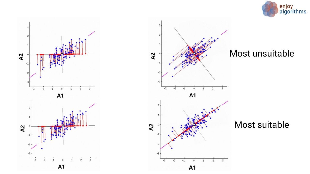
It's the scenario when the rotating line meets the purple lines (4th image of the most suitable case), which we call the case of maximum variance. So our first PC will be along the line, which passes through the two purple lines.

Similarly, the same procedure will be followed for the second PC to find the maximum variance but with an additional constraint that it should be perpendicular to the first PC. Eigenvalues and Eigenvectors help us find the same two dimensions. Eigenvectors are the unit vectors from the origin, which correspond to the directions along which the PCs will lie. Eigenvalues are the coefficients attached with eigenvectors that say about the variance carried along with corresponding eigenvectors.

#calculate eigenvalue and eigenvector
from numpy import linalg as LA
egn_values, egn_vectors = LA.eig(covariance)

For our dataset, eigenvalues and eigenvectors are given in the below images. Every row in the eigenvector matrix corresponds to one eigenvector. Please note that the magnitude of every eigenvector is 1 (unit vector), and they are perpendicular to each other.To check their orthogonality, we can perform dot product of vector_1 = [-0.73517866, -0.6778734]and vector_2 = [0.6778734, -0.73517866].If this product results in zero, then these vectors must be orthogonal.

We can calculate the amount of variance carried by any eigenvector using eigenvalues. 

From the above example, eigenvector_2 contains 96.3% (1.28402771 / (1.28402771+0.0490834)) of the variance present in the original dataset the 3.7% variance is along the eigenvector_1.

Step 4: Sort eigenvalues in decreasing order

Our first principle component (PC) will be the eigenvector corresponding to the highest eigenvalue will be our first principle component (PC). Similarly, our second PC will be the eigenvector corresponding to the second-highest eigenvalue. So to arrange the PCs in the most to least relevance index, we need to sort the eigenvalue, but it should be done such that we should not lose the information about which eigenvalue corresponds to which eigenvector. 

There are only two eigenvalues in our dataset, and the highest is 1.28402771. Hence eignevector_v2 = [0.6778734, -0.73517866]will be our first PC. As we already know, this PC will contain 96.3% of the total variance; we can ignore the rest, 3.7%. 

Note: We can choose to retain both dimensions as well. But to feel the reduction, we have decided to ignore the second PC.

What is Scree Plot?

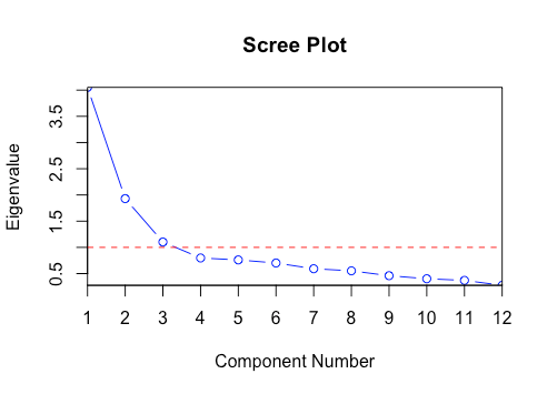
In multivariate statistics, the plot of eigenvalues with respect to PCs is known as Scree Plot. This plot is used in determining the number of PCs to retain. In the image below, PCs having eigenvalue > threshold (shown in red line) should be retained, and the rest can be discarded. This threshold can be considered a hyperparameter and tuned according to the project's needs.

Step 5: Forming the newer feature set along the principal component axes

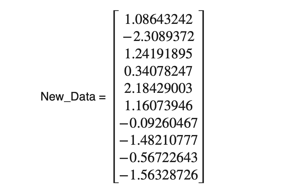
Once we have decided the number of components we want to keep, we need to form the matrix (also known as feature vector)with column entries as eigenvectors. As we already know, every row of the eigenvector matrix corresponds to one eigenvector. To form the feature matrix, we need to place the transpose of selected eigenvectors as column entries, e.g., [eigenvector1.T, eigenvector2.T, …., eigenvector_N.T]. Please note that we will use eigenvectors corresponding to those PCs only that we have selected to keep. In our case, we decided to keep 1 PC only to realize the reduction. Hence;

Data with reduced dimension would be,
NewData = Standardizeddata * feature_vector. 

#new attribute calculation
new_vector = np.matmul(Z3.T,egn_vectors[1:].T)

Standardized data would be the columns after standardizing the attributes of the original data.

Comparison with Scikit-Learn PCA implementation

The Scikit-learn framework has an in-built PCA algorithm where we need to pass the number of components that we want to retain and the data to be transformed.

from sklearn.decomposition import PCA
pca = PCA(n_components=1)
PCs = pca.fit_transform(Z3.T)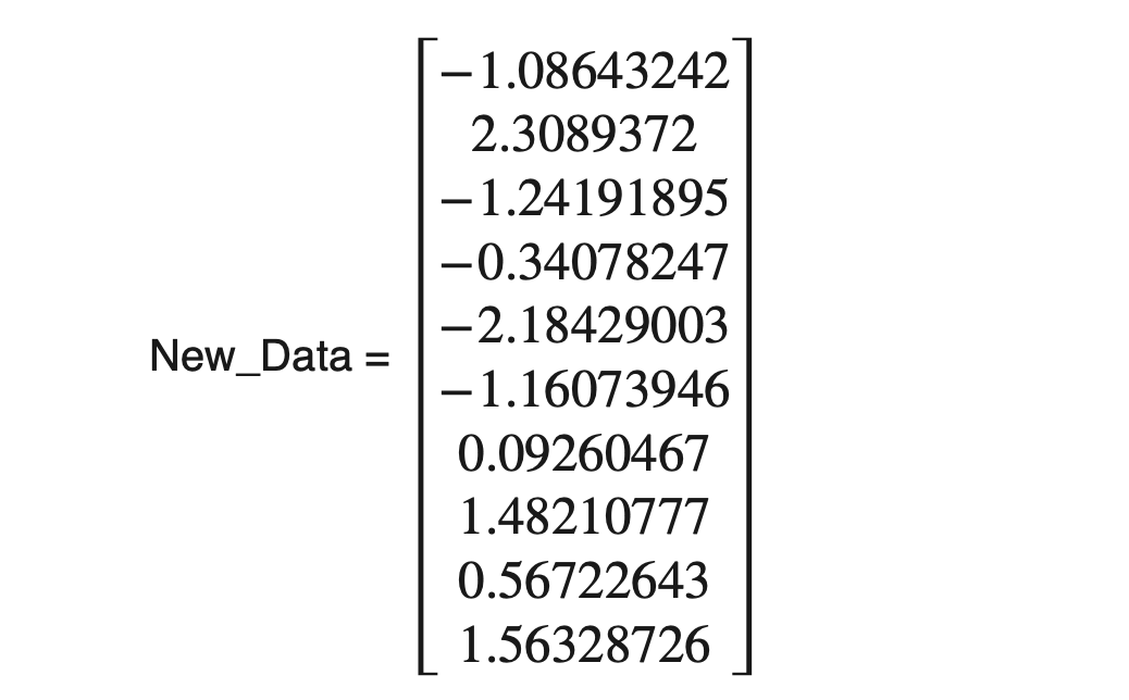

It is producing the same output as above but with the opposite sign.
Note: The sign of the entries in the new data can be the opposite because the eigenvector formed is a unit vector. It can be represented in both positive and negative directions. 

What are the assumptions we make in PCA?

We make certain assumptions while performing PCA on the feature set.

• The number of samples: Ideally, the number of samples in the data should be five times the number of features present.
• Features are correlated: We assume that the features present in the original set should be correlated so that the components formed after PCA preserves the originality.
• No outliers are present: Outliers can affect the overall variance of the data, and we know PCA gives importance to the features having high variance. Standardization generally solves the problem of outlier presence in the data, but removing outliers before applying standardization will be more helpful.
• Lower variance corresponds to lesser information: Components corresponding to lower eigenvalues are assumed to be noises and the most prominent candidates to be discarded.
• Linearity: Principal components should be a linear combination of the original features.

Where do we use PCA?

PCA is beneficial among machine learning engineers and data scientists. It is used for a variety of applications. Some of them are:

• Reducing the image size: We calculate the principal components of the image and remove components containing lesser information. This way, we reduce the image size, known as image compression.
• Facial Recognition: To reduce the complexity of the problem statement, we convert the facial images using PCA. The converted face is also called EigenFaces.
• Medical Science: A wider variety of problem statements use PCA. One of them is to detect the correlation between cholesterol and lipoprotein.

Additional Task to perform

Now we must practice our learning on a different dataset. One common Iris dataset (comes with Scikit-learn) consists of three different types of irises' (Setosa, Versicolour, and Virginica) petal length, petal width, and sepal length and sepal width, stored in a 150x4 numpy array. These flowers, sepals, and petals are shown in the image below.

As this dataset has four columns as features, [ Petal length, Petal width, Sepal length, Sepal width], we can not plot it ( 3 attributes can be plotted in 3D figures, but we can not plot 4D figures). Try to reduce the dimension of this dataset using PCA.

Possible Interview Questions

Some of the most asked interview questions on this topic are:

• What are Principal Components in PCA?
• What is the need for PCA in machine learning projects?
• What is the scree plot, and how did you tune the threshold?
• What does a covariance matrix represent?
• Is PCA affected by the presence of outliers?

Conclusion

In this article, we have implemented one of the most famous algorithms used for dimensionality reduction, Principal Component Analysis. We saw the steps involved in the PCA algorithm and compared the new features formed using our implementation and Scikit-learn's in-built implementation.

References

1. Principal Component Analysis: Siddhant Mishra, DOI:10.5455/ijlr.20170415115235
2. Principal component analysis: a review and recent developments: Ian T. Jolliffe, https://doi.org/10.1098/rsta.2015.0202

Enjoy Learning, Enjoy Algorithms!