Sentiment Analysis using Naive Bayes

Sentiment Analysis is a technique that comes under natural language processing(NLP) and is used to predict the emotions reflected by a word or a group of words. In this modern world where it has become complicated to predict people's state of mind, technologies like machine learning are helping a lot in monitoring the social media activities of the youth. While In 2004, Pang and Lee used Machine learning in sentimental analysis for the first time and achieved an accuracy of 86.4%, which was pretty good then.

Sentiment analysis is instrumental in brand monitoring, market research and analysis, social media monitoring, and many more. Companies like Google chrome, Apple, Twitter, and KFC use sentimental analysis for brand monitoring and customer service. We will discuss some of the use cases at the last of this blog.

Key takeaways from this blog

After going through this blog, we will have an understanding of the following things:

1. How is machine learning applied to sentiment analysis?
2. Naive Bayes for sentiment analysis.
3. Steps involved to build a sentiment analysis model.
4. Advancements in Naive Bayes.
5. Industry application of Naive Bayes.

Machine learning in sentiment analysis

Dealing with text data is one of the most rigorous work, and thinking of doing it manually will be a suicide. As of May 2020, on average, 6000 tweets are posted every second. So you can imagine the amount of data Twitter has to go through daily; therefore, we need a more effective and efficient approach to deal with it. Various algorithms and techniques are used for sentiment analysis; some are Support Vector Machine (SVM), Naive Bayes, and Linear Regression. In this blog, we will discuss one of the simplest probabilistic algorithms, Naive Bayes. Before going into detail, we will see how Naive Bayes works.

How is Naive Bayes used for sentiment analysis?

In Naive Bayes, probabilities are assigned to words or phrases, segregating them into different labels. As discussed in our previous blog, naive Bayes works on the Bayes theorem. Here we will understand Naive Bayes with the help of an example.

From the table above, a generative model like Naïve Bayes will try to learn how these sentiments are classified using the corresponding text. For example, it will see that a sentence having the word "good" has a high probability of being a positive sentiment. Using such a probabilistic value, a total probability of a test sentiment being positive or negative can be assigned.

Steps to build a Twitter-Sentiment analysis model

We have seen how Naive Bayes works, and now we will discuss steps to build a sentiment analysis model using the Naive Bayes algorithm. 

Step 1: Data Extraction/Collection

You can find many datasets of sentiment analysis on Kaggle. We are using Twitter Sentiment Extraction Dataset in this model.

Data Description

The dataset contains four columns and 27481 rows representing features and data samples.

• textID: unique ID's given to each data sample.
• text: tweets we have to perform analysis on.
• selected_text: the set of words having more weightage in calculating sentiment probability.
• Sentiment: nature of tweet (neutral, negative, positive).

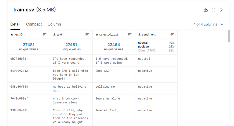
After describing the dataset, let's try to get a closer look at our dataset by visualizing it through various text analyzing tools.

Step 2: Exploratory Data Analysis 

Visualizing the data is of utmost importance before feeding it to the model. We will be using wordcloud and histogram to perform exploratory data analysis on the data.

Value counts

Visualizing number of samples categorized in positive(1), negative(-1) and neutral(0) using histogram.

twitter_df['sentiment'] = twitter_df['sentiment'].map({'positive': 1,'negative': -1,'neutral': 0},na_action=None)
count=sns.countplot(data= twitter_df, x= 'sentiment',order = twitter_df['sentiment'].value_counts().index)
plt.show()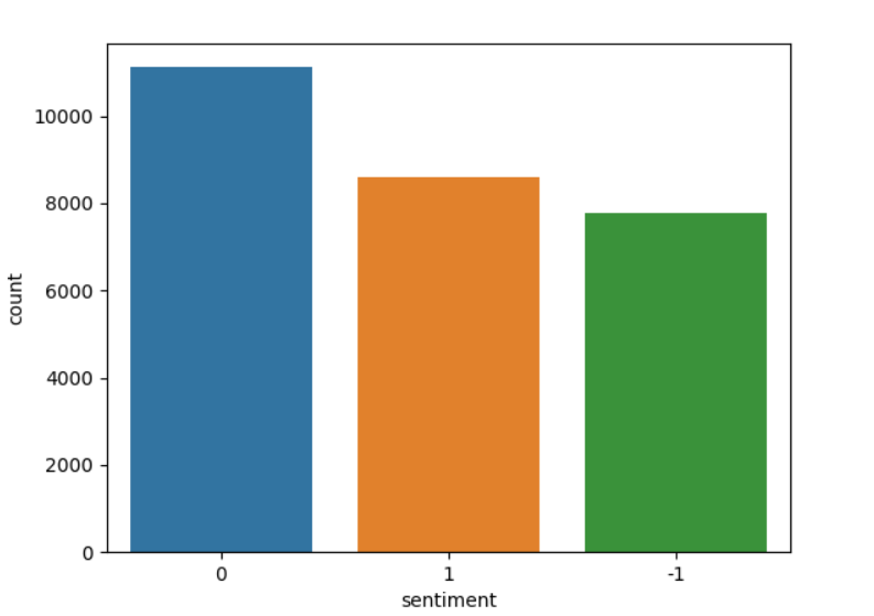

Wordcloud

Wordcloud represents the words present in data with variations in font size, increasing with frequent occurrences. In our 'label' feature, we have three positive, negative, and neutral sentiments so that we will form three wordclouds of each sentiment.

Positive sentiment wordcloud

positive = twitter_df[twitter_df['sentiment'] == 1]

plt.rcParams['figure.figsize'] = (10, 10)
plt.style.use('fast')

wc = WordCloud(background_color = 'orange', width = 1500, height = 1500).generate(str(positive['text']))

plt.title('Description Positive', fontsize = 15)
plt.imshow(wc)
plt.axis('off')
plt.show()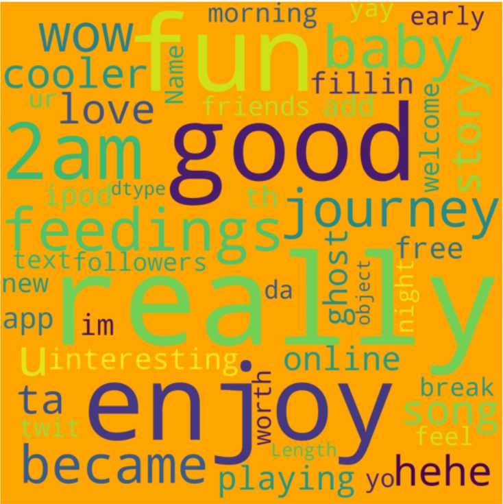

Negative sentiment wordcloud

negative = twitter_df[twitter_df['sentiment'] == -1]

plt.rcParams['figure.figsize'] = (10, 10)
plt.style.use('fast')

wc = WordCloud(background_color = 'orange', width = 1500, height = 1500).generate(str(negative['text']))

plt.title('Description Negative', fontsize = 15)
plt.imshow(wc)
plt.axis('off')
plt.show()

Neutral sentiment wordcloud

neutral = twitter_df[twitter_df['sentiment'] == 0]

plt.rcParams['figure.figsize'] = (10, 10)
plt.style.use('fast')

wc = WordCloud(background_color = 'orange', width = 1500, height = 1500).generate(str(neutral['text']))

plt.title('Description Neutral', fontsize = 15)
plt.imshow(wc)
plt.axis('off')
plt.show()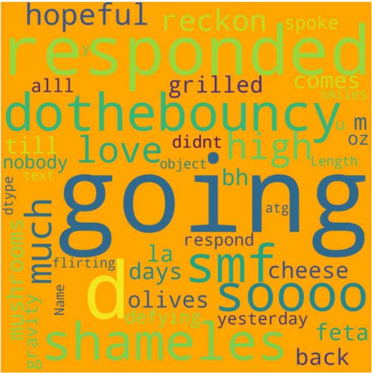

This will be sufficient to understand our dataset and move towards applying data preprocessing steps.

Step 3: Data Pre-processing

Natural language processing is the domain of machine learning that deals with text and voice data and ensures that the machine understands them in the same way humans do. In this blog, we analyze text data only, so we will only talk about text data preprocessing steps.

• Lowercasing: The first step is to lowercase the tweets to ensure the consistent flow of NLP tasks.
• Remove punctuations and hyperlinks: Punctuations and hyperlinks do not add any information to the tweets, so it is better to get rid of them.
• Remove Stopwords: Stopwords are English words that do not add much meaning to the tweet.
• Tokenization: Breaking down the sentence into words to form the vocabulary of comprehensive data.
• Stemming: This is a technique to group similar words by removing common prefixes and suffixes from tokenized words.
• Word Vector Encoding: This concept allows us to encode words into real-valued vectors such that words having similar meanings are clustered together.
• One hot encoding of target feature: We will encode the target variable using LabelEncoder().

You can check out this blog text data preprocessing for a detailed explanation and better understanding. I have attached the snippet of the code so you can have a look.

#--- removing punctuations, stopwords, hyperlinks and tokenizing ---
corpus = []

for i in range(0, len(x)):

  twitter = re.sub(r"@[A-Za-z0-9]+", ' ', x[i])
  
  twitter = re.sub(r"https?://[A-Za-z0-9./]+", ' ', x[i])
  
  twitter = re.sub(r"[^a-zA-Z.!?]", ' ', x[i])
  twitter = re.sub(r" +", ' ', x[i])
  
  twitter = twitter.split()
  
  ps = PorterStemmer()
  twitter = [ps.stem(word) for word in twitter if not word in         set(stopwords.words('english'))]
  twitter = ' '.join(twitter)
  
  corpus.append(twitter)
  
cv = CountVectorizer(stop_words='english')

x=cv.fit_transform(corpus)

This much cleaning of data is sufficient to build a decent machine learning model. Let's switch to model building.

Step 4: Model Building

Now that we have our dataset filtered and cleaned up, our model will be ready to predict test data output in the next two steps.

• Split the dataset: We can split our dataset to xtrain, xtest, ytrain, and ytest by importing train_test_split from sklearn.model_selectionlibrary.

from sklearn.model_selection import train_test_split

x_train,x_test,y_train,y_test=train_test_split(x,y,stratify=y,test_size=0.2,random_state=5)

• Creating an instance of the model: Import the MultinomialNB from the Naive Bayes module of the sklearn library using from sklearn.naive_bayes import MultinomialNB. Fit the model with xtrain and ytrain, and our model is ready to predict whether a tweet is negative, positive, or neutral. Hurray!

from sklearn.naive_bayes import MultinomialNB

model = MultinomialNB()
model.fit(x_train,y_train)

Step 5: Performance Evaluation

Since we have solved a classification problem, we will be using classification evaluation metrics for the performance analysis of our model. In general, if we have the confusion matrix, the accuracy from the confusion matrix does not give us an appropriate estimate of the model performance. Thus, it is good to use Precision, Recall, and F1-score for text-mining purposes to evaluate our model.

Accuracy score

The accuracy score is just the percentage of correct predictions in test data. For our model accuracy score is 75%.

Precision score

This metric is more concerned about false-positive cases and is calculated to penalize false-positive instances more. The precision score for this model comes out to be 75.37%.

Recall score

This metric is the opposite of the precision score and considers false-negative cases. It is also around 75% for our model.

F1 score

F1 score is the balance between precision and recall score. Since it maintains a balance and our recall and precision score were equal, this also comes out to be 74.8%

Excellent! we successfully built and evaluated our model. Now some improvisations can be made to make our model more accurate. It isn't easy to incorporate everything while building a model, but we recommend you try it. 

Improvizations in Naive Bayes

While this Naïve Bayes approach is not flawed in analyzing sentiments, further improvements can be made to increase its accuracy significantly. Let's look into some of those –

Binarization: Some frequent words in a text can increase the word count and probability, while actually, they have little significance in the decision-making process. To deal with that, binarization is done. Here is what binarization does –

As you have noted, the word count has been reduced for the marked word in the binarization text. Now, we will use the binarized text instead of the original in the same way we did for the Naïve Bayes example.

Sentiment Lexicon: Sometimes, the training data is insufficient to estimate the sentiment. In such a scenario, some word features can be added to the sentiment lexicon. This lexicon is pre-annotated with words that are already classified in the classes of the sentiment. When these words are encountered, a value can be added to that class for that word, given its annotation.

For example, the word 'good' can be pre-annotated as a word in the positive label. Whenever that word is encountered, an additional value should be added to the probability of sentiment being positive for having the word 'good'.

Now let's see how tech giants like Apple and KFC use sentiment analysis to boost their productivity.

Use Cases of Sentiment Analysis

Apple

Apple uses sentiment analysis to counter the opponent companies in the market. For example, Xiaomi launched a new phone, and users are complaining about heating issues after some time. Apple's team will find these defects by analyzing user comments and sentiment and using this information in their ad campaigns.

KFC

KFC mainly collects data from social media platforms like Youtube, Twitter, Facebook, and Instagram and uses Naive Bayes for sentiment analysis. KFC started to market its products using memes after a significant setback in its sales and analyzed the comments sentiments for the popularity check of its products and campaigns.

Bonus Section

Mathematical illustration of Naive Bayes

The equation for Naive Bayes is derived using the Bayes theorem:

With the assumption that all the features are independent of each other, the derived equation converts to:

Rewriting the derived equation for Naive Bayes in terms of our requirement:

label = Predicted sentiment; fi = ith word in the text

Or 

The below equation can give the probability of each word (w) given the class label(c) in a known vocabulary.

Let's do a small example from the book Jurafsky and Martin. Consider these statements:

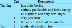
Sentiment Sample Case

There are five samples, of which three are negative while two are positive. So basically, given no other information, it is inherently biased towards the negative class. Let's analyze it a bit more –

But there is a problem, consider a widespread word, 'is'. The word is not present in any of the training samples, and if we use it to determine the probability of a sentiment given the word, it will result in zero for both cases. When multiplied by other probabilities, the entire result will be zero. To avoid this, an alternative is suggested as below-

This will assign a negligible probability value to words not encountered in either or both sentiments.

Using the above formula, the probability of a sentiment given the word can be computed.

Note that vocabulary in the sample case contains 20 different words, with 14 words in the Negative case and nine in the Positive case. |V| = 20. Note that repeated words are considered only once in the vocabulary.

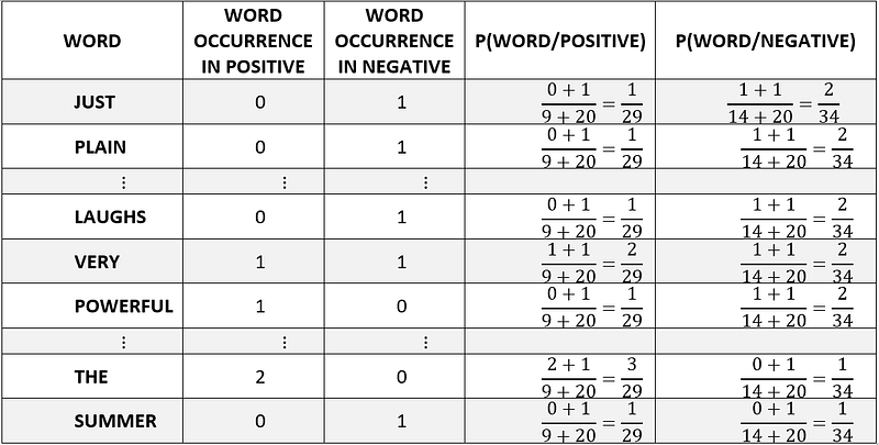
Word-Sentiment Probability Table

The table above represents the count of each word present in the vocabulary for both positive and negative labeled tweets.

Now working on the Test sample –

Words = [‘predictable’,’no’,’fun’]

The word 'with', having not been encountered in the vocabulary, is ignored.

Word-Probabilities:

Thus, the text probability in any particular class can be computed using the formulae:

Sentiment-Probabilities:

The predicted probability of negative is higher, so we classify the sample as negative. Using the same analogy and steps, we will try to build a sentiment analysis in the next part of this blog.

Possible interview questions on this project

Sentiment analysis is a classical project in the field of Natural Language Processing (NLP). If we have written this project in our resume, then the following questions can be asked in machine learning/ data science interviews:

1. What is sentiment analysis?
2. Why did you Naive Bayes algorithm? State some pros and cons for Naive Bayes.
3. What are the different evaluation metrics you used to evaluate your model?
4. What possible improvements can be done?
5. Explain the working of Naive Bayes in detail.

Conclusion

In this article, we used Twitter data of several users and demonstrated a step-wise process of implementing the Naive Bayes algorithm to predict the users' sentiment. We also discussed companies like Apple and KFC that use advanced sentiment analysis techniques to predict the users' demands and act accordingly. While building the model, we also saw some excellent text analysis techniques. We would highly recommend you to try this project. 

Enjoy Learning.