Introduction to Support Vector Machine (SVM) in Machine Learning

SVM is one of the most popular algorithms in machine learning and data science. Since the discovery of this algorithm in the 1990s, it has been widely popular among experts. The idea behind this algorithm is very intuitive, and experts consider this one of the best "Out of box" classifiers. In this article, we will try to develop the understanding of SVMs from a beginner to an expert level.

Key takeaways from this blog

• What is a Maximal Margin Classifier, and what is its relation with Support Vector Classifiers?
• What are Hyperplane, Support vectors, Margin, hard Margin, and soft Margin?
• What are the limitations of support vector classifiers, and how do Support Vector Machines overcome that?
• What is Hinge Loss?
• A basic implementation in python using Scikit-learn.

What is Hyperplane?

Humans have progressively designed geometry. First is the point, then there is a line on which that point lies. Then we have planes on which this line can lie. Hyperplanes are a popular concept in geometry that can be considered a generalization of "planes" in different dimensions. In 2D space, it's a line; in 3D space, it's a plane; in P dimensional space, it is a P-1 dimensional subspace.

As a fundamental nature, it separates the space into two parts. Let's consider the image below. Suppose X = [x1, x2, …., xn] is a vector in n-dimensional space, and βs are the coefficients. The left side of the image shows the R2 (Real) space (2 dimensions), where equation 1 is linear. On the right side, equation 1 is a plane equation in R3 space (3 dimensions). If a point satisfies equation 1, then it will lie on the line (in R2) (or on the plane (in R3)). Otherwise, it will satisfy either equation 2 or 3. Based on this inequality, we can decide on which side of the line (or plane) that point will be present.

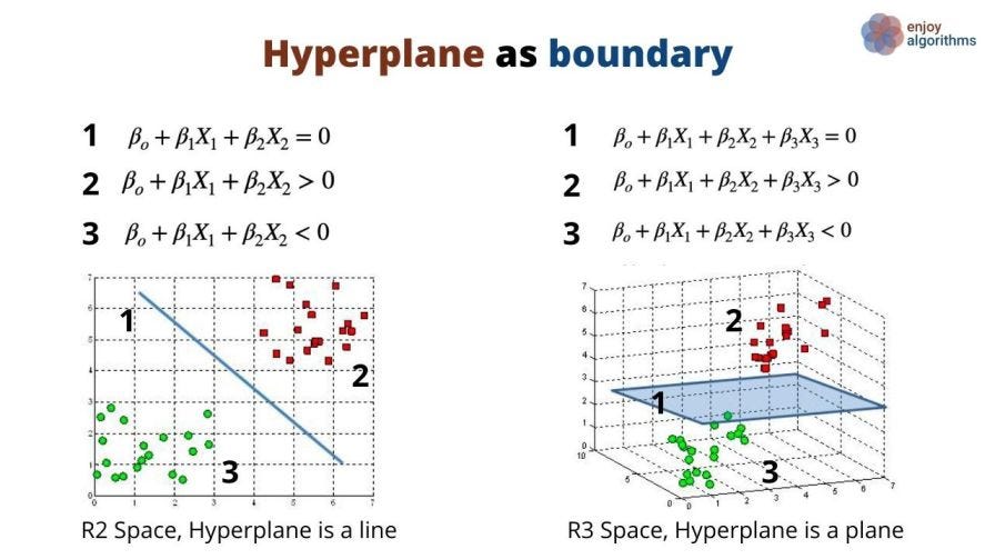
So basically, we can say that a hyperplane can act as a binary classifier that classifies points into two classes (+ve or -ve) based on the inequality that point follows. Let's consider the same example shown above. On the left side, if we can find the line equation (equation 1), we can segregate two types of dots (Red and Green), and the classification problem will be solved. Isn't it a trivial task to find the coefficients using linear regression or any other algorithm which can give us the coefficients to form the equation of that line? But there is a catch!

There can be infinite such lines, as shown in the image below. Which one do we have to choose?

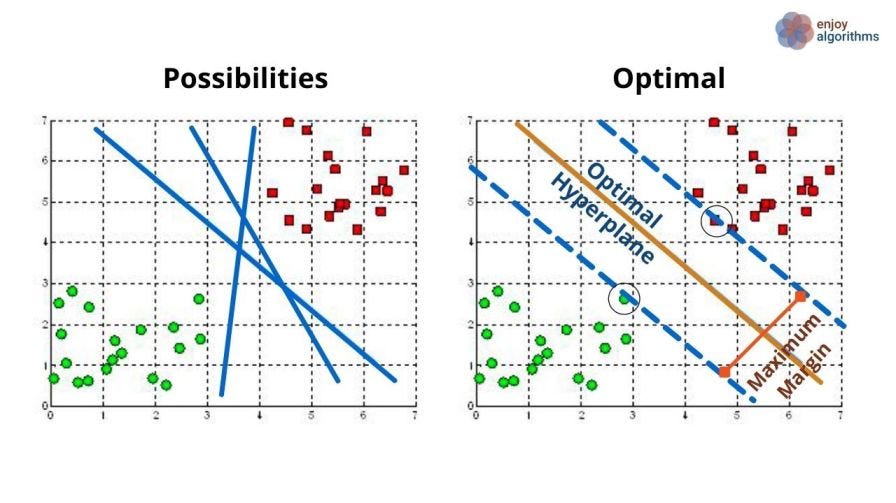
Here comes the concept of the Maximal Margin Classifier.

What is a Maximal Margin Classifier?

One natural choice for us can be selecting that hyperplane farthest from the training samples. The minimum of these distances from both sides of the plane will be called the Margin. Let’s say W1 and W2 are the margins from green and red dots, respectively. We want to maximize this Margin.

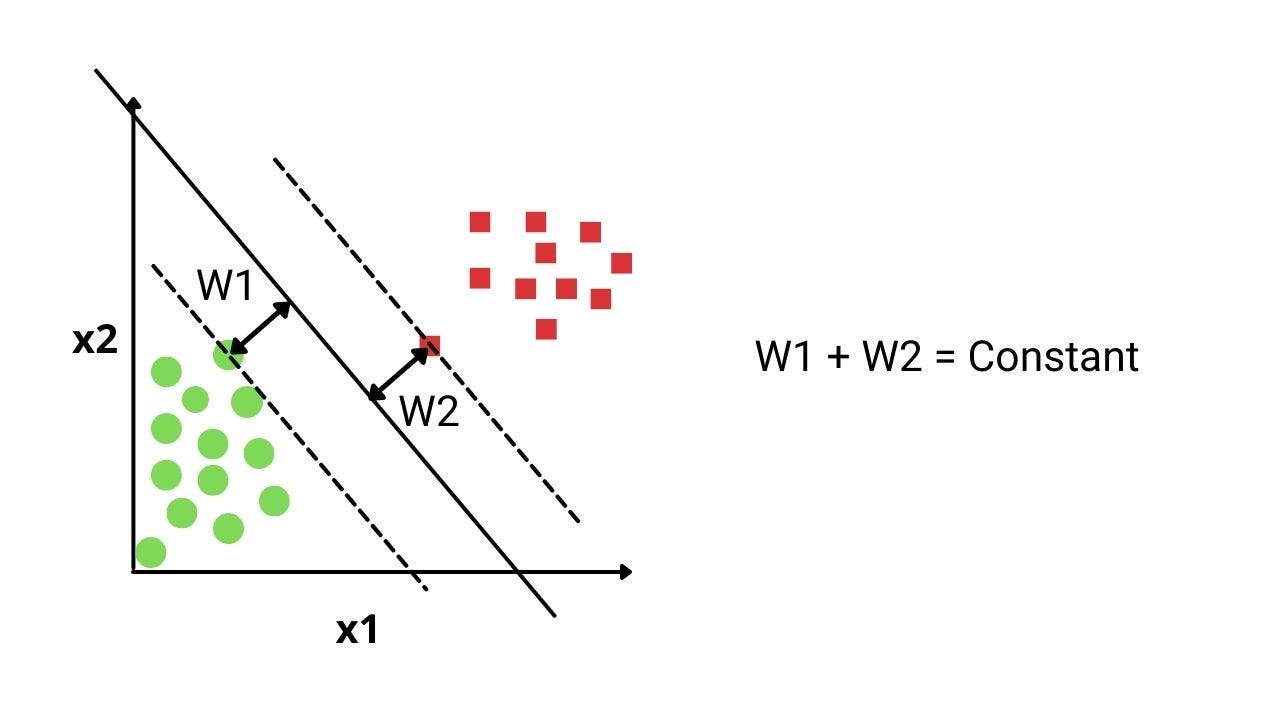
As W1 + W2 is constant, we want both W1 and W2 to be maximum. In such a scenario, W1 = W2 = W is the perfect and optimal distance. The hyperplane passing from this distance will be called the maximal margin hyperplane. In layman's terms, we can say that the maximal margin hyperplane represents the mid-line of the widest slab that we can insert between two classes represented as green and red dots.

So our overall objective is to fine-tune the coefficient values (β0,β1, β2,…, βn) so that W gets maximized. But we should take care of two "constraints":

1. All green and red dots should be present on the correct side of the line. In general, all training samples should be present on the correct side of the plane.
2. Distance between the maximal margin hyperplane and the training samples should always be greater than or equal to W (minimum margin distance) as we made W1=W2=W.

Let's say X = [X1, X2]' is a test vector from our test set. We need to put this vector in the hyperplane equation. The output value of the equation will decide the class of that test sample X. If positive, it will lie in the red category, and if negative, it will be in the green class. The output's magnitude is the vector's distance from the hyperplane. This distance is also regarded as the confidence score for the classification. The higher the distance, the better will be the confidence.

What is hard Margin?

The width of 2W ( W from class 1 and W from Class 2) is rigid, so we must not allow any single training sample to be present in this Margin. Because of this hard or rigid nature, we also called this Margin a Hard Margin.

But we can not expect data to be perfectly separable; hence the concept of hard Margin fails there. That's why we need softer margins. But before proceeding towards that, let's understand the support vectors.

What are Support Vectors?

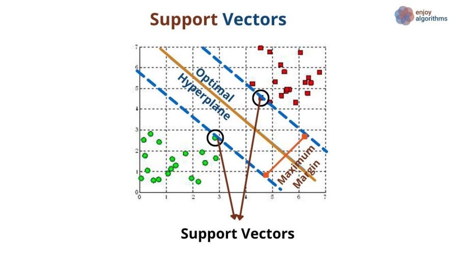
We noticed that only a few samples have a minimum distance from the hyperplane. These samples are the only contributing samples in estimating the maximal margin hyperplane. As those samples are p-dimension vectors, we call them Support-Vectors as they support the appearance of the hyperplane.

Why does SVM perform better even when the number of samples is lesser than the number of features?

One interesting thing to note here is that the maximal margin hyperplane only depends on the training samples' support vectors. The movement of other samples does not affect the hyperplane until and unless they cross the dashed margin lines. This is the sole reason for a better performance of SVM algorithms when the number of samples in the training data is lesser than the number of features. Now let's understand when this maximal Margin classifier fails. 

The Non-Separable case

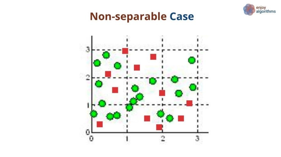
So far, we have discussed the case where the two classes were perfectly separable, and it was intuitive to separate them using a maximal margin hyperplane. But what if the training samples are not easily separable? In this scenario, a maximal margin classifier will not be able to classify or separate the two labels.

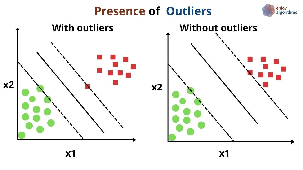
Also, what if the training samples, following the non-separable case, also contain some outliers or noise? These factors will affect the optimal or maximal margin hyperplane estimation. In the below figure, we can see how an outlier can affect the estimation of the optimal hyperplane. Without an outlier, the Margin will be maximum, and the model will be more confident about the predictions.

But what if we say that those shortcomings can be cured? What if we say that: It could be beneficial to misclassify some of the training samples to classify the remaining samples perfectly? Yes, that's right! Support Vector classifier does the same for us. Let's explore it in greater detail.

What are Support Vector Classifiers?

SVC allows some samples to be present on the Margin's wrong side or even the hyperplane's wrong side. While on the other hand, in the Maximal margin classifier, the Margin was hard, and it could not allow even a single sample to be present on the wrong side of the Margin. In the case of the Support Vector Classifier (SVC), the Margin is soft as it allows a few samples to be present on the wrong side but manages to maintain a higher margin. Hence, it is also called the Soft margin classifier.

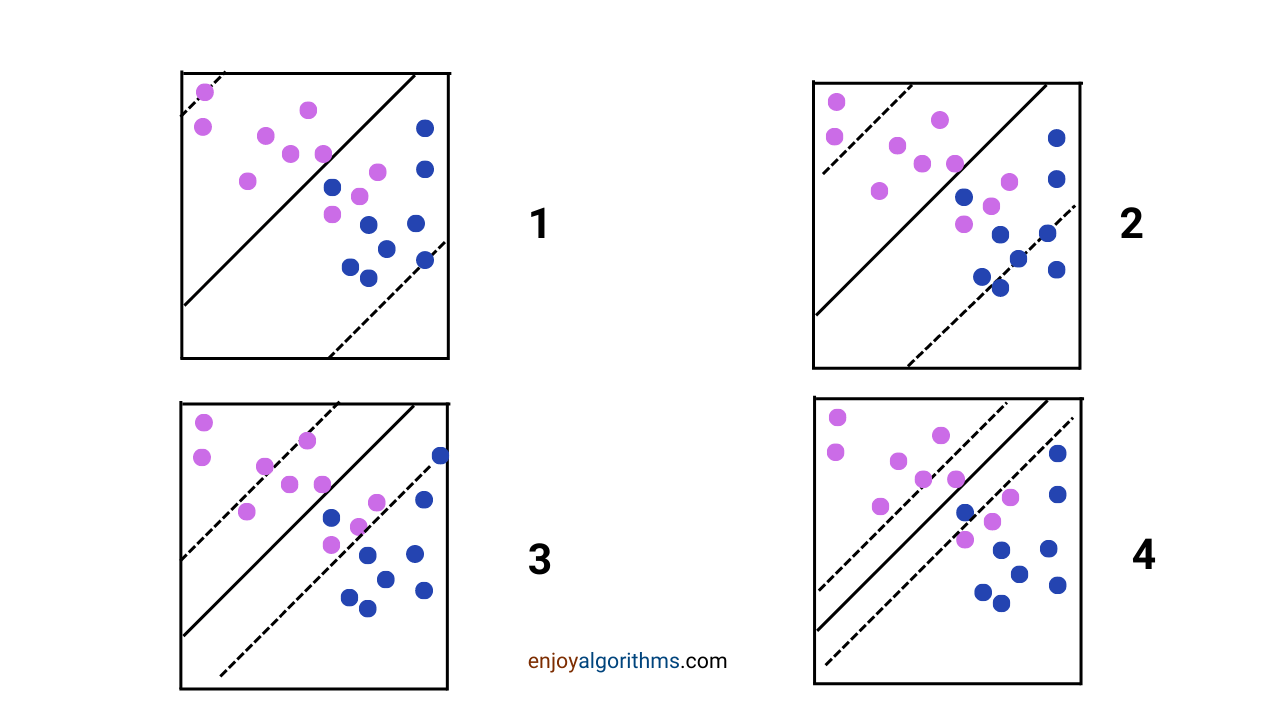
In the above figure, "1" has the softest Margin, which means a larger amount of samples can be present on the wrong side of the Margin. And "4" has the least soft Margin, allowing fewer samples to be present on the wrong side. The machine will try to optimize this trade-off and provide the optimal situation.

We can say that SVC has solved the problem of the Maximal margin classifier. But can we think of a situation where SVC won't perform better?

The case of Nonlinear Boundaries

For example, in the image below, there is an apparent circular decision boundary that is not separable by linear decision boundaries.

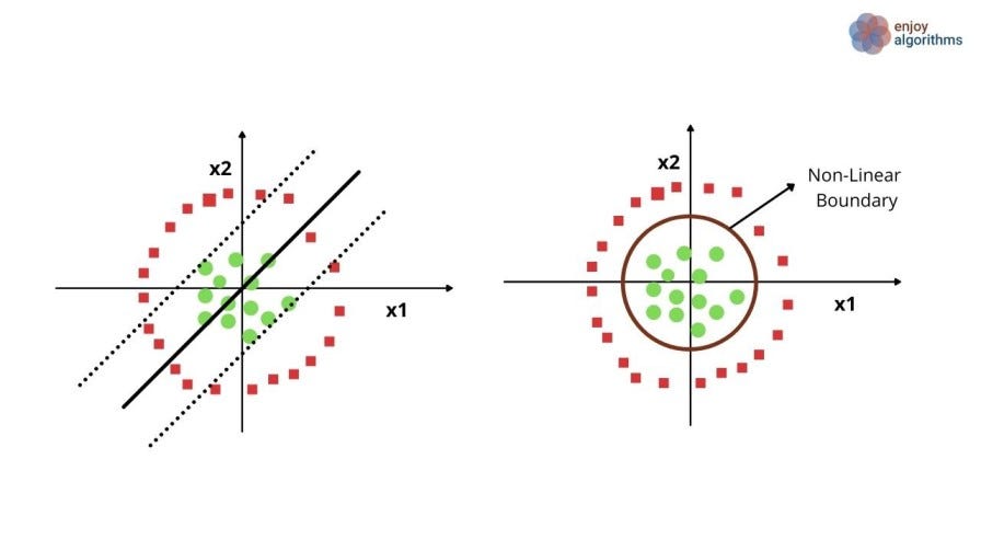
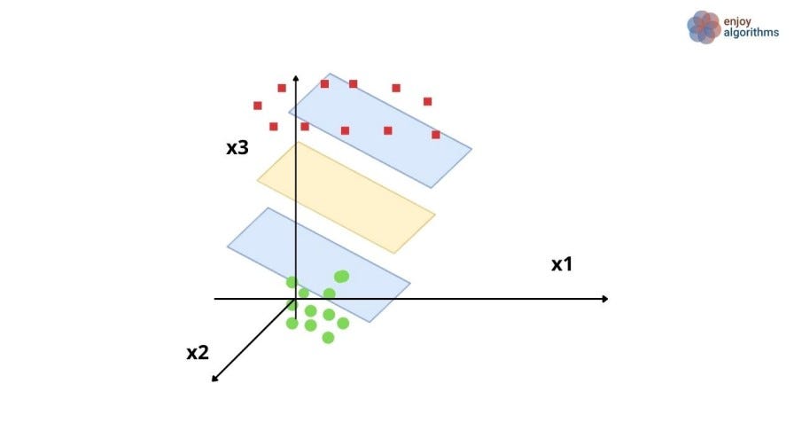
One of the solutions for this type of nonlinear decision boundary is increasing the "feature dimension" and separating labels using linear decision boundaries. For the above image, let's engineer one extra feature.

Now, in a 3-dimensional feature space, we can separate the labels using a 2-dimensional decision boundary.

Let's take another example where 1-Dimensional data is converted into 2-Dimensional space. In the image below, 1D data can not be separated by linear decision boundaries. But when we engineer a new feature as X2 = X1², we can find one.

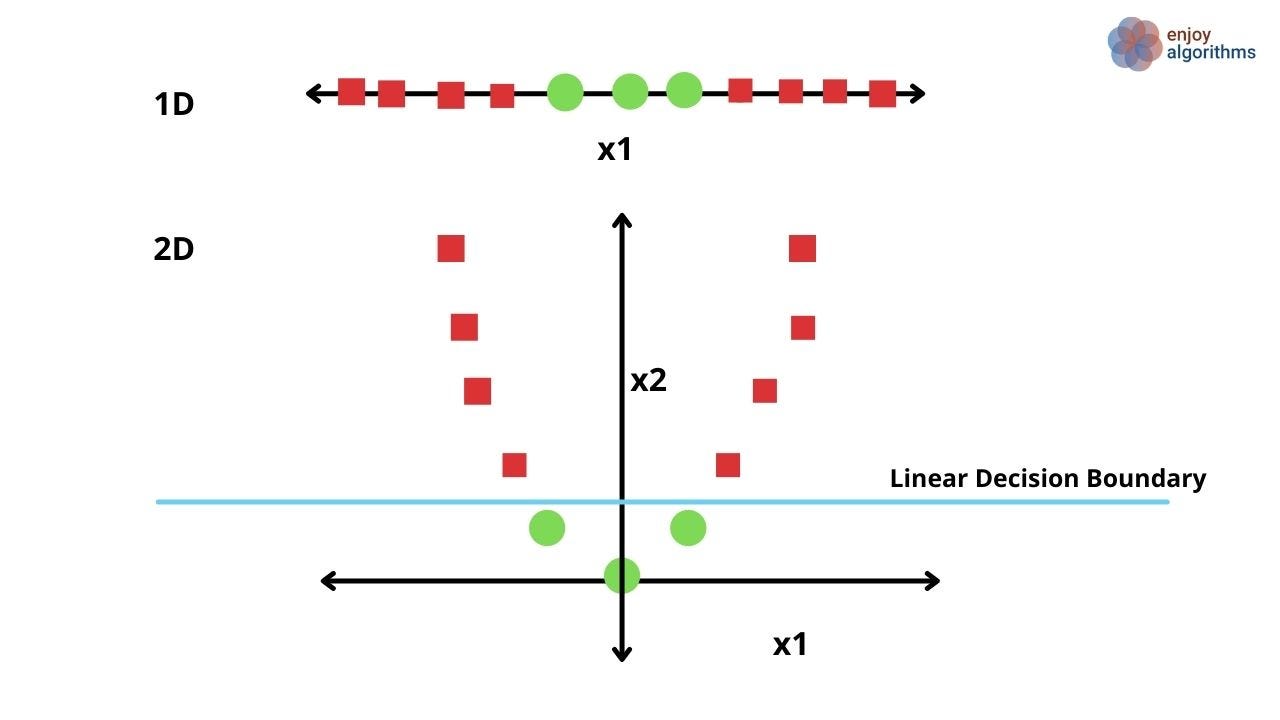
So finding the right kind of dimension increasing function to increase dimension is essential. But thousands of functions can be explored while finding it, and our program will never stop. There comes the rescuer, the Support Vector Machine.

What are Support Vector Machines?

An extension to the concept of Support Vector Classifier is introduced that enlarges the feature space in a specific way using "kernels" to provide a definite answer to the above question, a

From the above two examples, we must have learned that finding relationships among features is crucial to finding the extended feature space. One obvious intuition in this relationship between two vectors is finding the dot product of two vectors, which is perfect for sensing the linear relationships among vectors. But we can not just rely on the dot product as the relationship among features can be higher-dimensional. Hence, to generalize it, we write it as:

K is the generalized kernel function representing the relationship among different feature spaces. If K will be the dot product, this is also called a Linear Kernel function, and SVM will be the same as the Support Vector Classifier. We can design our kernel function as well according to our needs. Let's quickly explore some popular Kernel functions.

Linear Kernel Function

Dot Product of vectors X and X'.

Polynomial Kernel Function

The polynomial kernel function is a nonlinear kernel function with d>1 that gives more flexible decision boundaries w.r.t linear kernel function. Another nonlinear kernel function can be,

Radial Kernel Function

This is also called Radial Basis Function (RBF) kernel or the Gaussian kernel function. The value of γ states how influential every training example would be in deciding the new dimension. The higher value of γ considers lesser distant samples, and the smaller value will take more distant samples from the hyperplane.

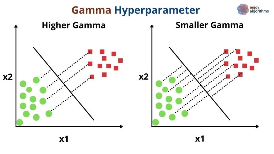
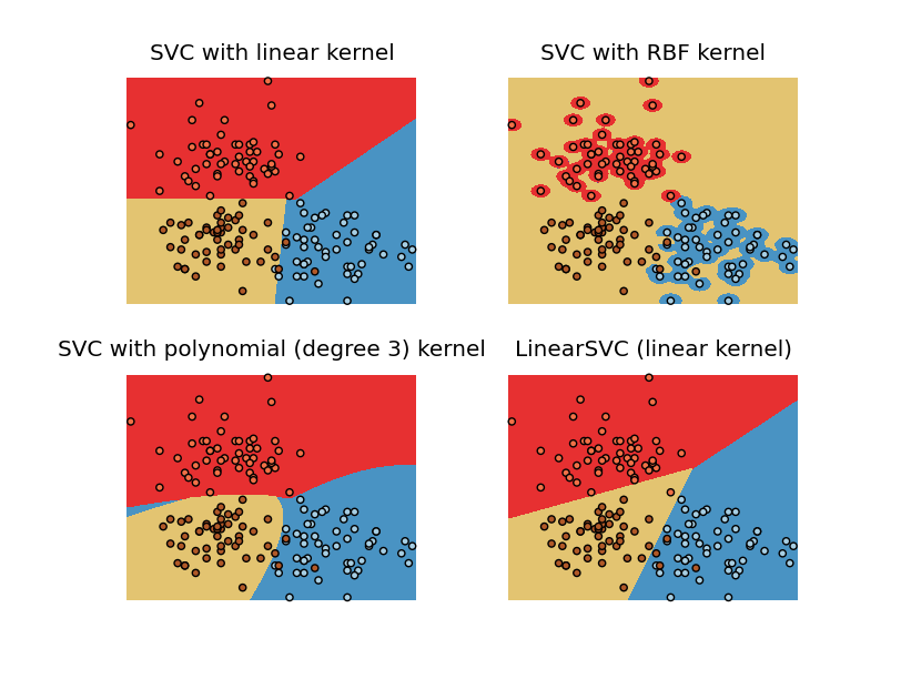
Source: StackOverflow

Too much theory, right? But one critical concept is still pending, "The Cost Function". We discussed that the goal of this algorithm is to find the parameters such that two objectives get fulfilled:

• Penalize the wrong predictions.
• Maximize the Margin. Or we can say that it penalizes the less confident predictions.

This goal differs from the rest of our objectives, like finding the parameters so that the error between predicted and actual Probability Distribution Functions becomes less. As the purpose is different, there is a need for a new cost function, especially for this case.

Cost Function For Support Vector Machine

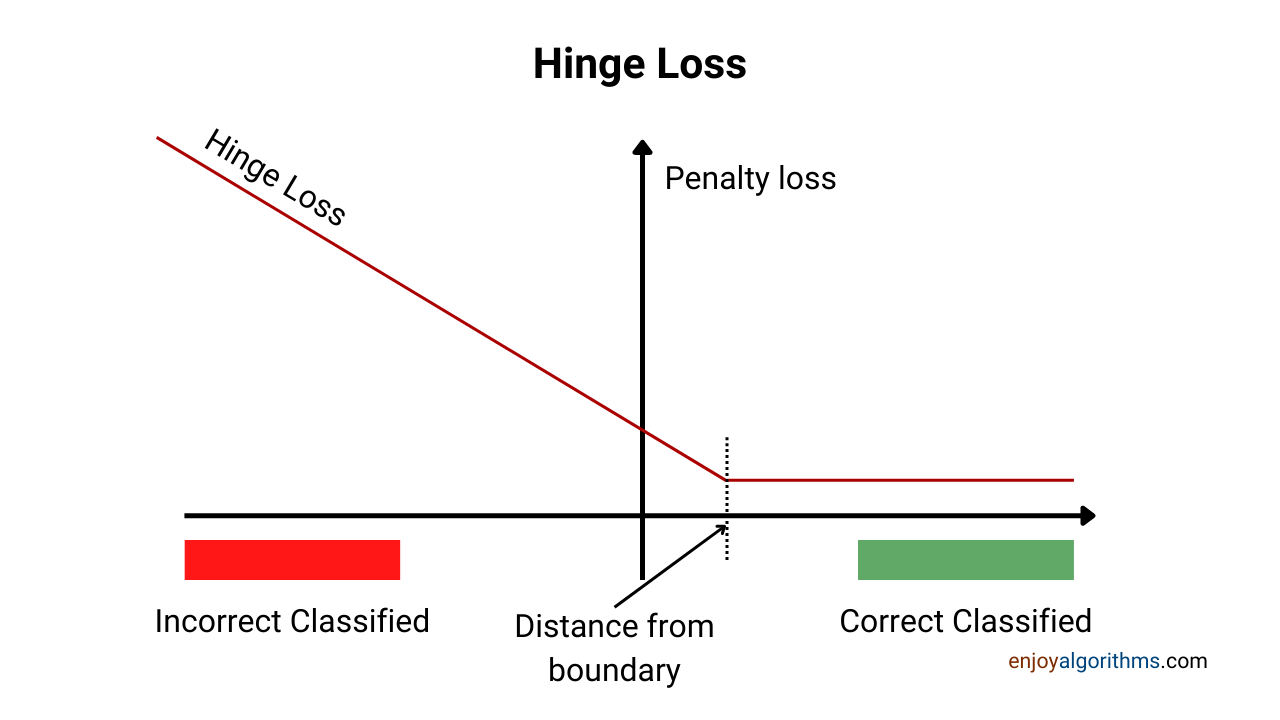
Our popular cost functions blog discussed the different cost functions for classification problems, like binary cross-entropy, categorical cross-entropy, and Hinge loss. In SVM, we use the Hinge loss cost function to find the parameters for our hyperplane such that the Margin becomes maximum and predictions become perfect. So let's explore this in detail. 

If we summarize our objective using the mathematical formulation, we can converge to something like the equation below:

For equation 1, βs are the coefficients of the hyperplane. Equation 2 is not a constraint but just a supportive factor for equation 3. If any point lies on the Hyperplane, means β0+ β1Xi1 + … + βnXin = 0, then k(β0' + β1'Xi1 + … + βn’Xin = 0) for any k ≠ 0. And the third line is the constraint for the maximal margin classifier that the perpendicular distance of any point Xi should be greater than or equal to the Margin. Can you guess which samples will be at least/equal distance to the Margin? 

By using the advanced statistical transformations, the above three equations got summarized in the equation below:

This is known as Hinge Loss. It is widely popular in the industry and the considered to be the reason for the success of SVM over a wider variety of problems.

We have seen too much theory now. Let's see SVM in real action now.

Step-wise Implementation of SVM on IRIS Dataset

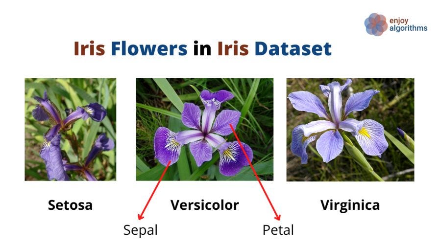
Here we will implement the support vector classifier with linear kernel function on the famous Iris dataset, which has three flower classes, Sentosa, Versicolor, and Virginica. We want to build a model which takes the input of petal length, petal width, sepal length, and sepal width and classifies the samples into three classes of flowers.

Step 1: Importing necessary libraries 

Here we need to import the basic libraries of Numpy, Pandas, and Matplotlib.

import numpy as np
import pandas as pd
import matplotlib.pyplot as plt

Step 2: Load the dataset

Here we will import the dataset, which is openly available and comes with the Sklearn library. After importing the data, we can perform fundamental data analysis by plotting the scatter plot of different input features and the target variables. It can be observed that there are three flower classes represented as [0, 1, 2].

from sklearn import datasets
iris = datasets.load_iris()            #loading dataset
X = iris.data[:,]                    #input
y = iris.target                      #target
iris_dataframe = pd.DataFrame(data=np.c_[iris['data'],iris['target']],
                             columns=iris['feature_names']+['target'])
plt.figure()
grr = pd.plotting.scatter_matrix(iris_dataframe, c=iris['target'],
                                  figsize=(15,5),
                                  s=60,alpha=8)
plt.show()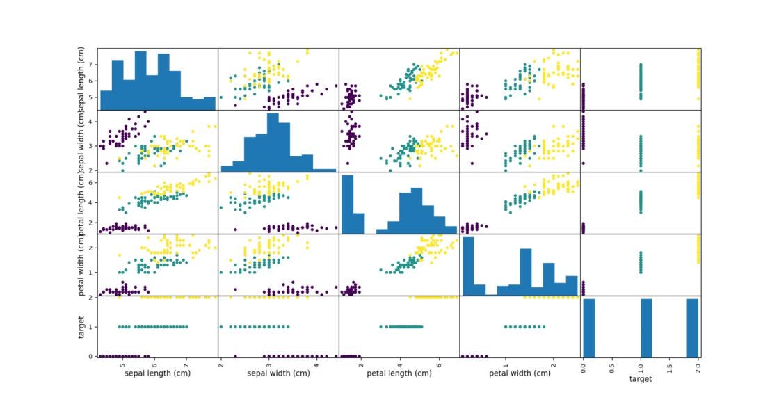

Step 3: Splitting the dataset and Standardizing it.

Scaling is always preferable before building a machine learning classification model with a Support Vector Classifier, as the decision boundary depends upon the support vectors.

X_train, X_test, y_train, y_test = train_test_split(X,y,test_size=0.25,random_state=0)

### Standardize the data
sc = StandardScaler()
sc.fit(X_train)
X_train_std = sc.transform(X_train)
X_test_std = sc.transform(X_test)

Step 4: Building the Model

This is the most crucial step where we will be training our classifier. If we look at the implementation of SVC in the Sklearn library,

sklearn.svm.SVC(*, C=1.0, kernel='rbf', degree=3, gamma='scale', coef0=0.0, shrinking=True, probability=False, 
                tol=0.001, cache_size=200, class_weight=None, verbose=False)

some important parameters need to be tuned to build this model,

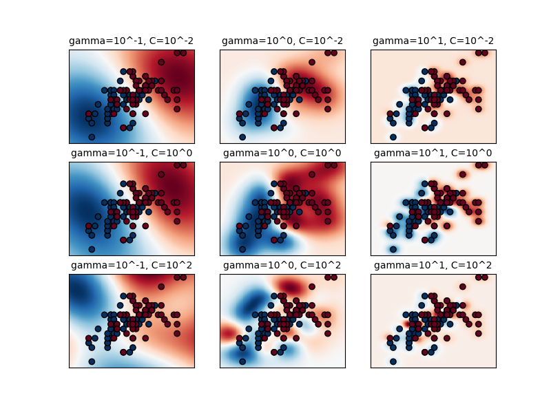
• C (Regularization parameter): This represents how much our SVC model is hard or soft.
• Kernel: We can design our kernel function. Some famous ones are RBF (default), poly, or linear.
• gamma (γ): This represents how much each training sample is influential in estimating the hyperplane.
• degree (d): In the above formula of the polynomial kernel function, degree shows the degree of the polynomial.
• probability: The default value is False. If we set it to true, our model will provide the probability for every class, and based on the higher confidence; we can select the correct class.
• shrinking: The default value is True and asks whether to use the shrinking heuristic or not. It shows optimization techniques for the SVM model and is advised to keep it true for performance benefits.
• random_state: The default value is None. It controls the pseudo-random number generation for shuffling the data for probability estimates. When probability = False, random_state is ignored.

#Create the SVM model
from sklearn.svm import SVC
classifier = SVC(kernel = 'linear', random_state = 0)
classifier.fit(X_train, y_train)
#Make the prediction
y_pred = classifier.predict(X_test)

The effect of C and γ can be seen in the image below:

Step 5: Evaluation of Built Model

Now we can evaluate the model by using the confusion matrix.

from sklearn.metrics import confusion_matrix

cm = confusion_matrix(y_test, y_pred)
from mlxtend.plotting import plot_confusion_matrix
from sklearn.metrics import accuracy_score

print(accuracy_score(y_test, y_pred))

fig, ax = plot_confusion_matrix(conf_mat=cm, figsize=(6, 6), cmap=plt.cm.Greens)
plt.xlabel('Predictions', fontsize=15)
plt.ylabel('Actuals', fontsize=15)
plt.title('Confusion Matrix', fontsize=15)
plt.show()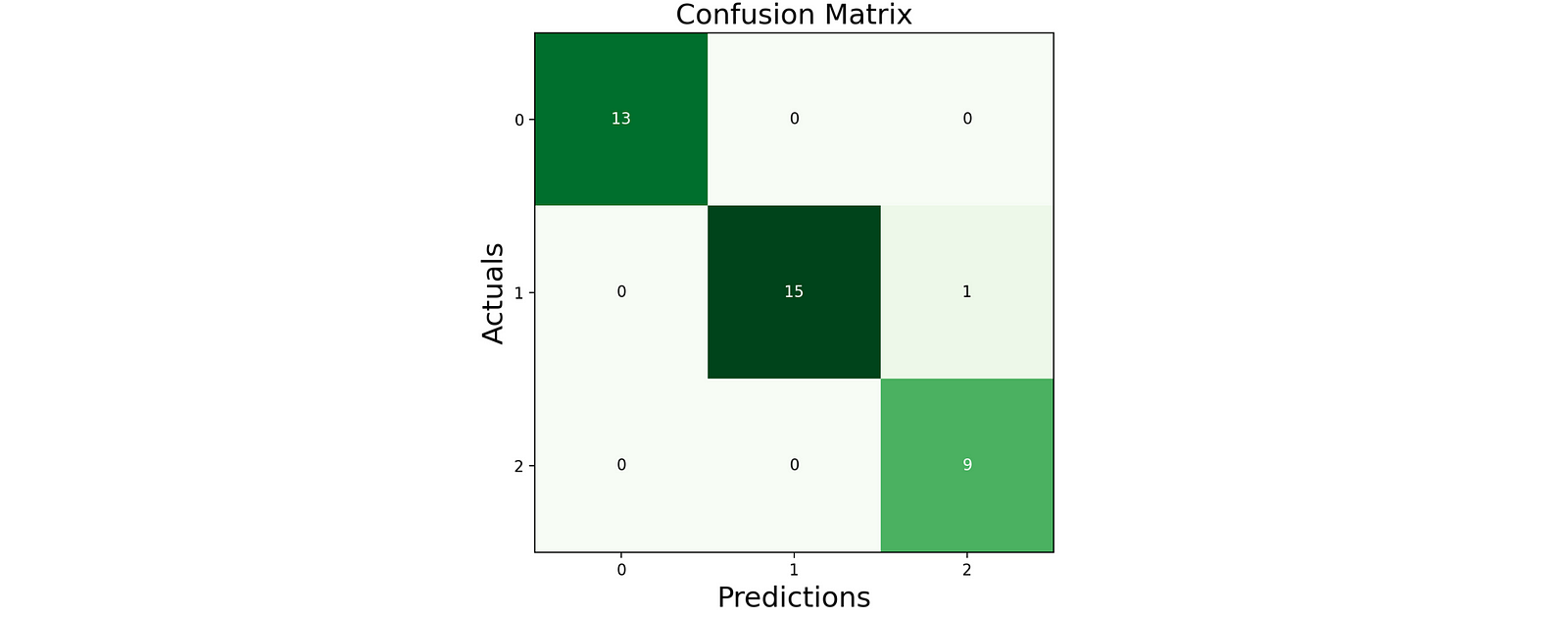

The accuracy of the test data is 97.3%.

Possible Interview Questions

SVM is one of the most asked topics in Machine Learning and Data Science Interviews. If we explore the different platforms like Glassdoor and Quora for the interview questions asked in bigger tech firms' interviews like Microsoft, we will find that most of the questions are related to SVM. Possible questions on this topic could be,

1. Explain the loss/cost function of the Support Vector Machine.
2. What are "support vectors" in a Support Vector Machine?
3. What's the role of Regularization parameter C in SVM?
4. What is the role of gamma (γ) in SVM?
5. What are Kernels in SVM?
6. What is a Margin, and what's the difference between Soft and Hard margins?

Conclusion

This article discussed an out-of-the-box classifier in Machine Learning, i.e., Support Vector Machine. We learned about hyperplanes, maximal margins, support vector classifiers, and support vector machines. We also learned about different kernel functions and implemented our SVM model on the famous iris dataset. We hope you enjoyed the article.

Enjoy Learning! Enjoy Algorithms!